a render of ice and fire (and more...)

Ya...this place has been like a haunted mansion for quite some while now. I did want to write some new stuff, interesting findings and readings for rendering every now and then, but just keep being lazy -___- This week though, I do feel I should write down some notes for the special occasion. After all, I don't think I will encounter this kind of experience that often in the next few years.

In the past 4 years, I had the privilege working on DreamWorks Animation's brand new path tracer MoonRay(Lee 17) , helped transitioning the studio rendering workflow from rasterization / point based global illumination to ray tracing. We delivered the first MoonRay full length feature film: How To Train Your Dragon: The Hidden World at the end of 2018 and presented to the world in 2019. Since then, I joined Walt Disney Animation Studio, working on its in house renderer Hyperion(Eisenacher13). My first credit in WDAS is Frozen2, and it will be in theatre 11/22/2019. Helping two extremely beloved IPs in the way I wish the most to contribute feels surreal every time I step back a bit and look at it: The first how to train your dragon is easily one of my all time top 5 animations, I still have goosebumps whenever watching it. I also vividly remembered the day Frozen released in 2013 Thanksgiving holiday time, went to Burbank theater with grad school classmate to support friends working on the title. As the song dropped, that "classic 90s Disney is back!" thought kept lingering til the end credit moment, and we had no idea how crazy (well maybe some...but definitely no where close to what really happened later...) the Frozen phenomena will invade the whole world in the next few years. As a rendering fan boy, shipping this two films with two participated renderers in two all star studios is a definite dream come true moment for me, truely grateful for the opportunities!

MoonRay team with How To Train Your Dragon Director Dean DeBlois

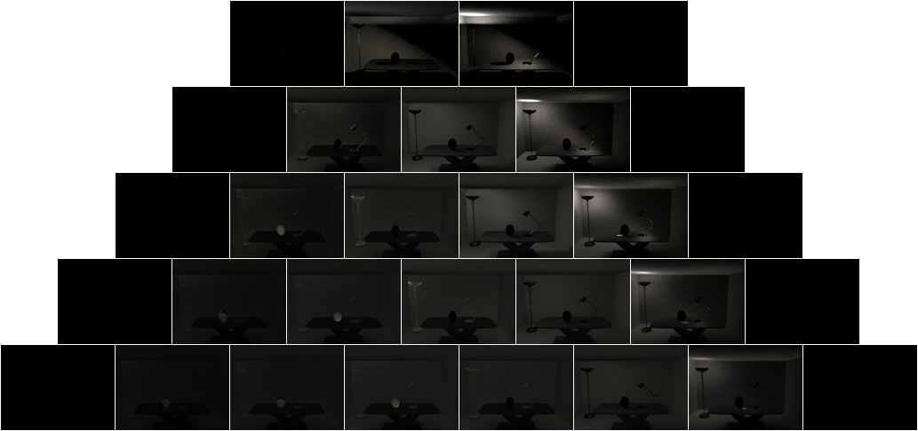
As a rendering software developer, my main contribution for MoonRay spans across geometry and volume. Geometry side: intersection kernels for curves/points/quadrics/instancing, rotation/deformation motion blur, tessellator for subdivision and polygon mesh, a geometry shader api separating geometry generation and internal renderer representation (shader writers can develop geometry shaders without touching renderer internal structure), a swiss army knife like alembic geometry importer (as demonstration of geometry shader api, turns out also become the major geometry work horse for movie production), primitive variables system (fx artists love to use this to pump in all sorts of arbitrary data into shader graph) , renderer scene graph for BVH construction/manipulation, and a lighters demanded artistic control feature: shadow linking. Volume side: volume integrator, (multiple) importance sampling for scattering/emission effects, multiple scattering, a light path expression syntax based volume aov system and a random walk subsurface scattering skin shader.

Production's first play of emissive volume: "it's expensive to converge...."

emissive volume + thin fog: my inner voice screamed in pain when watched the storyboard screening

The dust in the air has a term: CIA (craps in the air)

A mixture of particle and instancing (Brian: "do they simply want to break the renderer?")

Lightning in the gloomy cloud, because why not!?

"How many levels of instancing prim vars you need?" "Maybe 4? oops can you make it 8? We just passed that limit"

The earliest in production sequence for testing multiple scattering cloudscape

My current Hyperion responsibility is maintaining/improving the volume system researched/developed by Ralf Habel, Peter Kutz, Karl Li, Jan Novák and Patrick Kelly. Not one big shoes....Five big shoes to filled! Since both DWA and WDAS have presented their volume rendering system in SIGGRAPH already, I think it's safe to say here that the two renderers use two different algorithms: MoonRay uses classic decoupled ray marching (Kulla/Farjardo12) and Hyperion uses spectral and decomposition tracking (Kutz17) It is immensely fun to get my hands on two different volume algorithms and have a side by side comparisons for pros and cons of each other :). In the past year for Frozen2 production, my development work involves improving thin participating media scattering sampling efficiency, raw optimization for overall volume rendering speed, a general framework for volume aovs and improving volume shader editing interactivity for Hyperion.

You hear that Mr. Anderson? That is the sound of water splash with thousand bounces

Thick...white...emissive mist wall...purely brutal

A highly art directed shot that NUKE comes to rescue

Thin fog is actually surprisingly tricky for free path sampling

"Which renderer is the better one?" spicy question immediately dropped the first time I attended the volume rendering meeting in WDAS...whew...the room temperature is hot!...well I don't think it's is a fair apple to apple comparison though. My personal feeling is Hyperion aims for the most intense cases (million lights city night scene, thousand bounces multiple scattering cloudscape, full city of furry animal characters, 200GB+ geometry/texture for one shot....you name it!), MoonRay on the other hand tries to make the major cases extremely fast. One Octance VS Arnold = F1 VS Rally Car analogy in Internet sounds similar for this two renderers to me, though not to that extreme degree. Hyperion is one of the pioneer renderer leading the path tracing for film production revolution, and MoonRay's initiation/development was late by few years. This made Hyperion has the opportunity diving in difficult production problems in the first hand and thus a lot more research opportunities, while MoonRay steps on a lot less land mind pioneers helped detect/remove. Nothing right or wrong, just different approaches and styles, in different timing and with different resources.

The rendering field is not that big. When your tech lead won an Oscar and has been around the field for decades, there are quite some chances to meet celebrities in the field. ("Gonna head to the restaurant! Iliyan will join us for the lunch" "Uh....you mean that VCM Iliyan!?") As a shameless fan boy (the kind of fan boy that will ask selfie or autograph), it feels really cool to chat with rock stars, asking questions that I was puzzled while reading papers, or existing limitations when tried the algorithms on real life software. At the same time, when Alice Cooper said "Hang out with us!", it's probably still natural reaction for Wayne to feel this way

I can't help but constantly think I am under qualifying for this cool gig. There was one time that I pair programming with Thomas Müller, just made me keep thinking: "wow you can use 10 times my salary to hire this guy and it will be well worth the price!" There was another time when I asked Yonghao Yue for his free flight sampling spatial acceleration work, happenly Tzu-Mao Li and Yuanming Hu joined the chat. After few minutes I really felt I can't keep up my pace understanding three genius' conversation... It sounds kinda silly but finding my existing purpose in this field is a thought popping up every now and then for me. My current answer to myself: there are still unsolved problems for talented researchers to solve, and there are inevitably not that cool but important work for a production renderer to function. Before the holy grail shows up, someone needs to understand users' problems, come up solutions/workarounds for users under reasonable budgets/time, and that's my job and existing purpose.

"Any question that I may help to answer?" - Marcos Fajardo

"Yes. Can I have a picture with Mr. Arnold? :)"

For studio like WDAS and DWA that make cartoons, the mindsets for artists using renderers are still quite painter style. Striking a balance between flexibility, ease of use, performance and code complexity is a surprisingly involving, and ongoing daily negotiation/communication process. Some of my DWA colleagues volunteered to light few production shots, to better understand why the users request certain features. There are also times WDAS lighters demonstrate the lighting setup, composting Nuke graph breakdown, so the developers know what can be done, what can not be done in render. I found these back and forth communications extremely valuable for the features evaluation and prioritization. There are also some really good books talking about digital lighting, rendering from artists standpoint, I particularly like the book "Lighting for Animation: The Art of Visual Storytelling" since it also contains the process of how artists addressing notes, interviews revealing that different artists can approach the same problem with differnt styles, and what artists want for the future generation renderer (interesting but not that surprising, most artists in interviews want real time interativity, but not so much on physics/math correctness)

And there are those moments: the chats while sitting with artists waiting for the scene loading to see the first pixel, the gossiping with developers from other studio in conferences, really struck me as surprise (well maybe not that surprising when hearing another guy talk about it again): "Hey that's not what those marketing guys said!" I feel I can write it down since they are both informative and amusing.

"I am going to bias every pixel I render! why you tell me I should use an unbiased algorithm?" "well you can easily measure the error with ground truth...oh wait you probably don't care about that..." plus, what renderer is actually truely unbiased? you specify ray depth...bias! you use firefly clamping...bias! you use a denoiser...bias! Any photon mapping family integrator...bias! any sort of culling...bias! bias! bias! My feeling is: what artists want is predictable (consistent) result, unbiased...not that much. MoonRay once wants to remove ray depth control and the VFX sup came yelling at us: "stop! don't steal my render time controller!" "even that means energy loss?" "of course! it's far better than fireflies!"

"Will my ultimate one for all integrator ever come?" At the first wave of path tracing for film industry revolution there still seems to be quite some interesting variations between different renderers. We saw advanced integrators like SPPM, MLT, VCM, BDPT and even UPBP on Renderman and Manuka, and nowadays the heat of integrator arm racing in industry seems cool down quite a bit. Yes the statement of "the complexity of production renderer makes maintaining advanced integrator techniques impractical" sounds like sour loser playing guitar:"that guy only has technique, but his song has no soul", but I guess once signed up for the production rendering gig, I am already classified as sold out pop rock musician (shower though: WETA is probably the Dream Theater in this case). When you have multiple integrators in the renderer and you use the path tracer for 95% of time, chances are the time you need the advanced secret weapon that thing doesn't always stay consistent with path tracer (especially when you have so many artistic control knobs (hacks) on path tracer that may not implemented in other integrators) Path guiding became potential "path tracing killer" in the past few year, but I think we are still not there yet.

RenderMan removed UPBP support in recent 22.0 release

"Can't you just do this in comp?" "If I can do that in render I prefer getting it done in one pass" My fragile ego likes to hear artists prefer rendering solution instead of comp solution, but every time I got request like "I only want to change this part but left all the other stuff untouched" I tend to dodge it to NUKE (in DWA we even have the fathers of NUKE Jonathan Egstad and Bill Spitzak for this part of expertise). The last minute adjustment is super powerful weapon for artist and so far NUKE seems to be the best one providing the flexibility. Our MoonRay tech lead Brian Green once joked about: "we should aim for making the fastest aov renderer that can handle thousands of aovs if I knew how heavy artists are relying on NUKE" Recently renderer like Corona adds on more and more image processing functionality in renderer, maybe that can be a good alternative of putting all the functionality in 3D rendering land. So far on this kind of feature requests negotiation, I keep stepping back: "no I'm not going to put this witchcraft in our code!" "well if that doesn't make the code ugly maybe?..." "Fine...I'll do that if it doesn't slow the renderer down (too much)..."

"People will get sick of this physically based rendering look in the next few years, and people will start advocating stylized rendering...like what we did in the last renderer..." "Meh...stop making excuse because we are incapable of doing the right thing!" And then Spider-Man: Into the Spider-Verse came, snatched the Oscar. While in theater, I felt I witnessed a part of history, and feel bad to the colleague made that prophecy :P  I am always not the bsdf guy in the team so I feel I can't make that much comment here. Personal take: For look development, physically based shading provides predictable/consistent render across different lighting scenario. For lighting, you still want to have the per shot, per light adjustable backdoor to make director happy. Keep bsdf consistent. Keep light flexible.

"Uhh...how long does it take for this shot to load up so I can debug this ticket?" "You know what Wayne? I think all you rendering developers should at least once have this kind of taste to understand how miserable our life is! In some crazy shots it took more than an hour for us to see the first pixel!" When Max Liani presented XPU in SIGGRAPH2018 he pointed out: we can shoot out more and more rays when hardware advances, but the increasing loading time keep taking over all the time saved from ray tracing. For artistic iteration, we hope at least we only need to load the shot once and keep modifying it without relaunching the renderer. Depends on how much the renderer relying on precompute cache and the quality of BVH, this is not always possible though. There will never be fast enough renderer for artists. You give painters unlimited time, they'll change the painting everyday since they never feel it's good enough. For farm render, if artist need to go home and check the render tomorrow, whether it's 10 hours or 5 hours doesn't matter that much, only when you can get the time  below 3 hours (Blizzard's Redshift workflow) so artists can have two dailies in an day that will change the workflow.

With all unsolved problems still on the road, I feel extremely lucky to be able to stand in the front row watching this ongoing rendering revolution. The TOG paper from Sony Arnold , Solid Angle Arnold , WETA Manuka , Disney Hyperion,  Pixar RenderMan reveal so much information that was once not easily accessable, and the community people are so open to each other nowadays. It is a wonderful time to work on rendering :) Thanks all the friends and comrades at work (I am shy to say that at work, but Joe, Karl and Mark I am your big fan!) I hope I can keep helping artists making beautiful/inspiring movies to entertain you, and add some more contents to this ghost town.

Thanks Shenyao for supporting the movie in day 1 :)

Bidirectional Path Tracing 9 - Some images and postmortem

This test scene, is a clumsy attempt to reproduce that famous Veach rendering: a scenario where large portion of the lighting contribution coming from indirect lighting, and the lights are not directly visible from eye. This makes the chance to construct a path from eye extremely difficult while the reverse way (light tracing) serves a much better purpose.

The original scene in Veach97

My modeling skills are so terrible that I don't bother to hurt people's eye with a self modeling scene. The model courtesy:
http://3dsky.org/3dmodels/show/stol_christopher_guy_serra_1
http://3dsky.org/3dmodels/show/lampa_massive
http://3dsky.org/3dmodels/show/torshier_blake_a4711pn_1br

left: path tracing with 36 spp

right:bidirectional path tracing with 25 spp

(around the same rendering time)

This scene is almost like incurable cancer for unidirectional path tracing to converge. On the other side, bidirectional path tracing shows really promising result with less amount of the sample (around the same rendering time though, we do a lot more occlusion test in bidirectional scenario compare to path tracing). Even we crank sample up to something crazy:

left: path tracing with 10000 spp

right: bidirectional path tracing with 6400 spp

(around the same rendering time)

path tracing is still noisy while bdpt pretty looks pretty clean already. The following image shows the unweighted contribution of all the different strategies (yes, it is a tribute to original paper too :) )

And the following image shows the weighted contribution of all the different strategies:

And a clean render with larger resolution using bdpt:

I'll try to be honest though, even the bdpt roughly get implemented step by step according to the original paper. There are still a considerable amount of TODO in the list that should be get in there

When a bug goes unnoticed during a presentation

1. The dipole style BSSRDF does not work in bidirectional path tracing right now. As my earlier post  mentioned: dipole integration is an area+solid angle 4 dimensional integration compare to regular bsdf 2 dimensional integration. Whether dipole integration work, how does it work, how to combine...this all remains pretty vague to me still. I have a feeling that the true volume integration style subsurface scattering can integrated with bdpt better, but that is just a guess still.

2. Volume integration does not work in bidirectional path tracing right now. I can't even say my unidirectional path tracing volume integration is in complete stage now (it does work for homogeneous volume, but that's it, and it's a single scattering ray marching model....). There are some resource talking about the bidirectional path tracing volume integration  But just be frank, it's not in the current version of implementation.

3. Image based lighting does not work in bidirectional path tracing right now. My unidirectional implementation contains something I felt clever back in that time but kind of regret at this moment: it does mipmap selection based on the solid angle pdf (based on this article ) The implementation converge faster compare to the naive 2D cdf version, but it also causes bias while changing the sampling number. Before I fixed this biased implementation, I have no plan to move on to get it supported in bidirectional path tracing.

4. Normal/Bump map shading normal cause incorrect result in the current bidirectional path tracing. This is actually stated in Veach97 actually spend a whole chapter talking about this (Chapter5 The Sources of Non-Symmetric Scattering) The implementation should be pretty straightforward but I just didn't put into it yet.

5. Chapter 10.4 Reducing the number of visibility tests is skipped totally at this moment.

6. Better s=1 case handling. In unidirectional path tracing, there are some clever ways to optimize local direct lighting samples when we are aware of the intersection geom information (for example, the lighting samples from back side of the geometry can totally be ignored) The current implementation doesn't support this at all. It will require some pdf tweaks also as Veach97 stated in 10.3.4.2 )

The bdpt journey was quite fun and challenging alone the way, it forces me to brush up lots of math topics that I though I understood but actually not. It did really impress me about how math/algorithm plays an important role in the rendering side (even strong as Disney Hyperion, they did mention they would try to avoid indoor indirect lighting in production shot if possible) bdpt doesn't look like a really coherent algorithm if just using the naive implementation (I think this is the debate happen in that first post when WETA/Disney hold different opinions on the rendering architecture design), and it would be really interesting...to see if the future research would spend time optimize it in a coherent way. :)

Bidirectional Path Tracing 8 - Combine multiple s,t strategies optimally

Now we have all the s,t combination strategies implemented, which means for a certain path length integration we can have multiple solutions to apply:
path length 1: 3 ways to integrate direct visible light
path length 2: 4 ways to integrate direct lighting
path length 3: 5 ways to integrate 1st bounce lighting
path length 4: 6 ways to integrate 2nd bounce lighting

Simply added all the strategy would result to overbright image (probably 3 times brighter direct visible light, 4 times brighter direct lighting, 5 times brighter 1st bounce lighting....etc) But does simply divide by strategy number work? Something like:

\(C_{s+t=2}(\bar{x}) = 1/3(C_{s=0, t=2}^{*}(\bar{x})+C_{s=1, t=1}^{*}(\bar{x})+C_{s=2, t=0}^{*}(\bar{x}))\)

\(C_{s+t=3}(\bar{x}) = 1/4(C_{s=0, t=3}^{*}(\bar{x})+C_{s=1, t=2}^{*}(\bar{x})+C_{s=2, t=1}^{*}(\bar{x})+C_{s=3, t=0}^{*}(\bar{x}))\)

\(C_{s+t=4}(\bar{x}) = 1/5(C_{s=0, t=4}^{*}(\bar{x})+C_{s=1, t=3}^{*}(\bar{x})+C_{s=2, t=2}^{*}(\bar{x})+C_{s=3, t=1}^{*}(\bar{x})+C_{s=4, t=0}^{*}(\bar{x}))\)

\(...........\)

Uhh...... it might work......when you have a camera with intersectable lens + every light in the scene is intersectable + no specular bsdf in the scene, which means: any Dirac distribution light (point/directional/spot lights), bsdf(specular), camera(pinhole camera, orthogonal camera) can break this naive divide method. The reason is, some of the strategy just can't handle certain Dirac distribution: s=0 strategies can't handle point light since ray will never hit the light, t=0 strategies can't handle pinhole camera since ray will never hit the lens, t=1 strategies can't handle direct visible specular surface since \(f_{s}(\omega_{o}, \omega_{i}) = 0\) for every possible \(\omega_{o}, \omega_{i}\) combinations. (We rely on sample bsdf specifically for specular bsdf to get a \(f_{s}(\omega_{o}, \omega_{i})\) that represent the whole integration result in Dirac distribution case)

The above image show the length 4 strategies for specular bsdf + pinhole camera (from left \((s=0, t=4)\) to right \((s=4, t=0)\) ) Divide by 5 is definitely not enough to serve the purpose of combing length 4 strategies here.

Even we assume we won't encounter Dirac distribution, assign equal weight to each strategy doesn't provide the optimal result anyway. We see that certain strategy work particularly good on certain scenario, it doesn't make sense to add in other inferior strategy in this scenario to downgrade the result. The problem is: how we know which strategy work best on which scenario?

Veach95 introduced multiple importance sampling to solve this problem. The sampling combination techniques were applied to several rendering related topics includes: direct lighting sampling, final gathering, and bidirectional path tracing. Lafortune publish bidirectional path tracing around the same time with Veach, but the paper didn't formalize the way to combine different sampling strategies. My personal feeling is that bdpt become a powerful beast after applying multiple importance sampling. It was cool to come up result with multiple strategies, but determine which strategy is better in run time is mind-blowing cool :P

The multiple importance sampling estimator:

$$F=\sum_{i=1}^{n}\frac{1}{n_{i}}\sum_{j=1}^{n_{i}}\omega_{i}(X_{i,j})\frac{f(X_{i,j})}{pdf_{i}(X_{i,j})}$$

where \(n\) is the number of sampling techniques, and \(n_{i}\) is the number of sample for technique \(i\). With the power heuristic approach Veach propose:

$$\omega_{i} = (n_{i}pdf_{i}(X_{i,j}))^2/\sum_{k=1}^{n}(n_{k}pdf_{k}(X_{k,j}))^2$$

For example, we got a length 3 path come up with \((s=2,t=2)\) strategy, and we would like to have its MIS weight. What we need will be figure out the pdf to form this path with other strategies \(P_{A}(\bar{x}_{s=0, t=4})\), \(P_{A}(\bar{x}_{s=1, t=3})\),  \(P_{A}(\bar{x}_{s=3, t=1})\),  \(P_{A}(\bar{x}_{s=4, t=0})\) The \(n_{i}\) can simply be treated as 1 since we form every strategies for each integration samples. Expand the result:
$$\omega_{s=2,t=2}(\bar{x}) = \frac{P_{A}(\bar{x}_{s=2, t=2})^2}{P_{A}(\bar{x}_{s=0, t=4})^2 + P_{A}(\bar{x}_{s=1, t=3})^2+ P_{A}(\bar{x}_{s=2, t=2})^2+P_{A}(\bar{x}_{s=3, t=1})^2+P_{A}(\bar{x}_{s=4, t=0})^2}$$

Veach97 use the notation \(k=s+t-1\) and \(p_{i} = P_{A}(\bar{x}_{s=i, t=s+t-i})\), rewritten path \(\bar{x}_{s,t}\) as \(\bar{x} = x_{0}...x_{k}\). This simplify the power heuristic equation to \(\omega_{s,t} = \frac{p_{s}^{2}}{\sum_{i}p_{s}^{2}}\) . In above equation:
$$\omega_{s=2,t=2}(\bar{x}) = \frac{p_{2}^2}{p_{0}^2 + p_{1}^2+ p_{2}^2+p_{3}^2+p_{4}^2}$$
where:
\(p_{0} = P_{A}(x_{3})P_{\omega^{\perp}}(x_{3}\rightarrow x_{2})G(x_{2}\leftrightarrow x_{3})P_{\omega^{\perp}}(x_{2}\rightarrow x_{1})G(x_{1}\leftrightarrow x_{2})\)

\(\:\:\:\:\:\:\:\:\:P_{\omega^{\perp}}(x_{1}\rightarrow x_{0})G(x_{0}\leftrightarrow x_{1})\)

\(p_{1} = P_{A}(x_{3})P_{\omega^{\perp}}(x_{3}\rightarrow x_{2})G(x_{2}\leftrightarrow x_{3})P_{\omega^{\perp}}(x_{2}\rightarrow x_{1})G(x_{1}\leftrightarrow x_{2})P_A(x_{0})\)

\(p_{2} = P_{A}(x_{3})P_{\omega^{\perp}}(x_{3}\rightarrow x_{2})G(x_{2}\leftrightarrow x_{3})P_{\omega^{\perp}}(x_{0}\rightarrow x_{1})G(x_{0}\leftrightarrow x_{1})P_A(x_{0})\)

\(p_{3} = P_{A}(x_{3})P_{\omega^{\perp}}(x_{1}\rightarrow x_{2})G(x_{1}\leftrightarrow x_{2})P_{\omega^{\perp}}(x_{0}\rightarrow x_{1})G(x_{0}\leftrightarrow x_{1})P_A(x_{0})\)

\(p_{4} = P_{\omega^{\perp}}(x_{2}\rightarrow x_{3})G(x_{2}\leftrightarrow x_{3})P_{\omega^{\perp}}(x_{1}\rightarrow x_{2})G(x_{1}\leftrightarrow x_{2})\)

\(\:\:\:\:\:\:\:\:\:P_{\omega^{\perp}}(x_{0}\rightarrow x_{1})G(x_{0}\leftrightarrow x_{1})P_A(x_{0})\)

All ingredients (\(P_{\omega^\perp}\),  \(P_{A}\), \(G\)) can be collected during the path building stage. In fact, Veach even did a clever optimization to avoid duplicate computation between different \(p_{i}\):
$$\omega_{s,t} = \frac{p_{s}^{2}}{\sum_{i}p_{s}^{2}}=\frac{1}{\sum_{i}(p_{i}/p_{s})^{2}}$$

By treating the current \(p_{s}=1\), we can come up the other \(p_{i}\) related to \(p_{s}\) using the equation:

\(\frac{p_{1}}{p_{0}} = \frac{P_{A}(x_{0})}{P_{\omega^{\perp}}(x_{1} \rightarrow x_{0} )G(x_{1} \leftrightarrow x_{0})}\)

\(\frac{p_{i+1}}{p_{i}} = \frac{P_{\omega^{\perp}}(x_{i-1} \rightarrow x_{i}) G(x_{i-1} \leftrightarrow x_{i})}{P_{\omega^{\perp}}(x_{i+1} \rightarrow x_{i}) G(x_{i+1} \leftrightarrow x_{i})}\) for \( 0 < i < k \)

\(\frac{p_{k+1}}{p_{k}} = \frac{P_{\omega^{\perp}}(x_{k-1} \rightarrow x_{k}) G(x_{k-1} \leftrightarrow x_{k})}{P_{A}(x_{k})}\)

and on the reverse side:
\(\frac{p_{0}}{p_{1}} = \frac{P_{\omega^{\perp}}(x_{1} \rightarrow x_{0}) G(x_{1} \leftrightarrow x_{0})}{P_{A}(x_{0})}\)

\(\frac{p_{i-1}}{p_{i}} = \frac{P_{\omega^{\perp}}(x_{i} \rightarrow x_{i-1}) G(x_{i-1} \leftrightarrow x_{i})}{P_{\omega^{\perp}}(x_{i-2} \rightarrow x_{i-1}) G(x_{i-2} \leftrightarrow x_{i-1})}\) for \( 1 < i \leq k \)

\(\frac{p_{k}}{p_{k+1}} = \frac{P_{A}(x_{k})}{P_{\omega^{\perp}}(x_{k-1} \rightarrow x_{k}) G(x_{k-1} \leftrightarrow x_{k})}\)

There are......some devils hidden in the details that need special treatments.

First, while reusing the path by connecting different path vertex from light path and eye path, the end point pdf need to be reevaluate since the connection changes the outgoing direction:

Second, \(\frac{p_{k+1}}{p_{k}} = 0 \) when \(p_{k+1}\) is a camera with Dirac distribution (pinhole camera) since there are 0 chance you can hit a pinhole camera.

Third,  \(\frac{p_{0}}{p_{1}} = 0\) when \(p_{0}\) is a light with Dirac distribution (point light, spot light....etc) since there are 0 chance you can hit a point/spot light.

Fourth, when \(x_{j}\) stands for a surface point with specular bsdf, \(p_{j} = 0\) and \(p_{j+1} =0\) Veach97 contains a detail explanation of this exception handling in 10.3.5, the basic idea is, when \(p_{j} = 0\):

\(\frac {p_{j}}{p_{j-1}} = \frac{P_{\omega^{\perp}}(x_{j-2} \rightarrow x_{j-1}) G(x_{j-2} \leftrightarrow x_{j-1})}{P_{\omega^{\perp}}(x_{j} \rightarrow x_{j-1}) G(x_{j} \leftrightarrow x_{j-1})}\) contains a \(P_{\omega^{\perp}}(x_{j} \rightarrow x_{j-1}) \) in denominator which is a number that is not an actual pdf but a hack to get integration working, let's just call it evil alien number for now

\(\frac {p_{j}}{p_{j-1}}\frac {p_{j+1}}{p_{j}} =\frac{P_{\omega^{\perp}}(x_{j-2} \rightarrow x_{j-1}) G(x_{j-2} \leftrightarrow x_{j-1})}{P_{\omega^{\perp}}(x_{j} \rightarrow x_{j-1}) G(x_{j} \leftrightarrow x_{j-1})} \frac{P_{\omega^{\perp}}(x_{j-1} \rightarrow x_{j}) G(x_{j-1} \leftrightarrow x_{j})}{P_{\omega^{\perp}}(x_{j+1} \rightarrow x_{j}) G(x_{j} \leftrightarrow x_{j+1})}\) evil alien number still sticks in denominator :|

\(\frac {p_{j}}{p_{j-1}}\frac {p_{j+1}}{p_{j}}\frac {p_{j+2}}{p_{j+1}} =\frac{P_{\omega^{\perp}}(x_{j-2} \rightarrow x_{j-1}) G(x_{j-2} \leftrightarrow x_{j-1})}{P_{\omega^{\perp}}(x_{j} \rightarrow x_{j-1}) G(x_{j} \leftrightarrow x_{j-1})} \frac{P_{\omega^{\perp}}(x_{j-1} \rightarrow x_{j}) G(x_{j-1} \leftrightarrow x_{j})}{P_{\omega^{\perp}}(x_{j+1} \rightarrow x_{j}) G(x_{j} \leftrightarrow x_{j+1})}\frac{P_{\omega^{\perp}}(x_{j} \rightarrow x_{j+1}) G(x_{j} \leftrightarrow x_{j+1})}{P_{\omega^{\perp}}(x_{j+2} \rightarrow x_{j+1}) G(x_{j+2} \leftrightarrow x_{j+1})}\) 

The interesting thing happen, another evil alien number \(P_{\omega^{\perp}}(x_{j} \rightarrow x_{j+1})\) appears in the nominator. To make thing even more interesting, this two number are actually the same number that can cancel each other. Yes I questioned myself once whether this two number is the same number and the result is true. In pure specular reflection case (mirror) there are both 1. In reflection/transmission combine material like glass, depends on the implementation, it may be 0.5 (giving half half chance to do the transmission or reflection), it may be a \(F(\omega_{o}, \omega_{i})\) Fresnel number so that you can do a bit importance sampling for this bsdf. 0.5 is self explanatory enough that pdf from \(\omega_{o}\) to \(\omega_{i}\) is the same as  \(\omega_{i}\) to \(\omega_{o}\). Fresnel number if you examine the equation carefully, pdf from \(\omega_{o}\) to \(\omega_{i}\) is still the same as  \(\omega_{i}\) to \(\omega_{o}\) :) 

The conclusion: a specular surface point  \(x_{j}\)  will bring an evil alien number to pdf \(p_{j}\) and \(p_{j+1}\) that this two pdf shouldn't be counted in the final weighting calculation, but as long as we move on to  \(p_{j+2}\), everything goes back to normal.

With the above gotcha in mind, here is my implementation of multiple importance sampling weight evaluation:

And this is how the above first bounce strategies looks like after assign appropriate MIS weight:

You can see the high variance noise (estimator with low pdf) got smooth out and different strategies only preserve the estimator result that with high pdf. The most important thing is: the added on result, still converge correctly compare to the Mitsuba reference.

battle royale round 3: bdpt rendering vs path tracing Mitsuba reference

One thing to notice is that even this scene is not a particularly fun one, bdpt already show that it can use much less samples converging to similar result path tracing did (the above comparison, bdpt use 196 spp, Mitsuba reference uses 400 spp) Though the rendered images are kinda boring (cornell box all the way til the end :P ) The bidirectional path tracing is roughly complete now, and I have to say, OMG!......this journey is definitely not a piece of cake for myself. Time to open up a beer for a small celebration! In the next post, I would try to come up some relatively more interesting images and do a postmortem of this round of implementation.

Bidirectional Path Tracing 7 - Implement every s,t combination strategies

After implemented t=1 strategy light tracing and visually verify the result can converge to s=1 path tracing, I move on to implement t=0 strategy light tracing: shooting ray from light and bounce around the scene until it slams on camera lens. This is probably the worst strategy generally when lens is small compare to the scene since it has so little chance the sample can hit the lens. It can't even render anything if the camera is a pinhole model since ray will never intersect a infinitely small camera lens (just like s=0 strategy never works when the bouncing ray try to intersect a point light) But we are going to implement every strategy anyway, so I would like to prove this strategy can converge (when there are enough amount of samples) to correct result.

One small new things to add is that I need to implement disk geometry to simulate camera lens (you didn't implement disk geometry!? @@  yup....I live in the sphere and polygon mesh world for quite some while) so that ray can hit it. It was a small quadric exercise and there it is:

One good thing for t=0 strategy is that you don't need to implement shadow ray testing since you never connect light pah with eye path. The code logic looks simpler and each sample is cheaper to evaluate as the result, still....it is really really slow to converge compare to t=1 light tracing and s=1 path tracing....reallllllly sloooooooow!

This is how it looks like in a simple dof scene with 100 samples

Crank it up to 10000 samples per pixel, still noisy....

The Mitsuba right side path tracing reference uses around 200 spp

Two strategies work, now move to implement all different strategies, which is the first 50% of bidirectional path tracing. The rough idea is: we create a path from light, we create a path from camera, we connect every end points of light path and camera path to form paths with different strategies and evaluate the unweighted contribution \(C_{s,t}^{*}\) . For example, to render a 2 bounces render, we need to integrate paths with maximum length 4. We generate a length 4 path from light, we generate a length 4 path from camera, and we can connect the end points of two paths to form the following strategies:

length 1 : (s=2, t=0), (s=1, t=1), (s=0, t=2) direct visible light

length 2 : (s=3, t=0), (s=2, t=1), (s=1, t=2), (s=0, t=3) direct lighting

length 3 : (s=4, t=0), (s=3, t=1), (s=2, t=2), (s=1, t=3), (s=0, t=4) 1st bounce lighting

length 4 : (s=5, t=0), (s=4, t=1), (s=3, t=2), (s=2, t=3), (s=1, t=4), (s=0, t=5) 2nd bounce lighting

It's a bit of waste but I do throw away the combination that is longer than the specified max path length. I feel this makes the code logic looks cleaner and rendering behavior more consistent (there won't be path length 5 result added into render when specified max length 4 in this implementation) Since there can be multiple strategies to generate a path, simply added all the strategies to the final render image will result to a over blown image. The first draft of implementation add mDebugS, mDebugT flags to specify which s, t to be added into the final rendering. This is actually a good debug resource since I can specify a particular light path to render and isolate down whether the bug only happen in specific path. The implementation of eval contribution for every s, t combination is wrapped in BDPT::evalContribution:

The constructEyePath and constructLightPath are really similar that I just list one of them in the following code segments. In the beginning I was planning to wrap this two as one utility function but the slight difference stops me to do that in the first try, maybe it should be refactored to one in the long rung:

and here are some images only display 1st bounce lighting for debug purpose during the development:

s=1, t=3 first bounce for glossy material

s=2, t=2 first bounce for glossy material

s=3, t=1 first bounce for glossy material

the above debug images will converge when we cranked up the sample number, but even in this simple setup we can tell different strategy have different converge speed compare to other strategies. In the above images, s=1,t=3 path tracing strategy seems to be the better strategy compare to the other two. How we determine which strategy is good for which scenario, and which strategy is better for other scenario? This is where multiple importance sampling come to rescue :) and I'll try to talk about my interpretation in the next post.

Bidirectional Path Tracing 6 - Implement light tracing

Like path tracing have s = 0 (trace ray from camera til it hits the light) and s = 1 (trace ray from camera, connect the ray intersection with a light sample) strategies, light tracing also have t = 0 (trace ray from light til it hits the lens) and t = 1 (trace ray from light, connect the ray intersecgtion with a camera lens sample) strategies. My first light tracing implementation was t = 1 strategy, mainly because it can handle edgy case that t = 0 strategy can't handle, ie, pinhole camera. (you can't hit a point light if you use s = 0 strategy right? ;P ) Also, when the lens is a really small object in the scene, it is way easier to connect a sample from the lens then try to hit the lens, which means, the t = 1 strategy generally converge faster than the t = 0 strategy.

The implementation is really straightforward once we have the \(C_{s,t}^{*}\) equation in the previous post. We set up a max path length (the level of bounces, 2 for only direct lighting, 3 for one bounce, 4 for two bounces....etc) then we evaluate \(C_{1,1}^{*}\), \(C_{2,1}^{*}\), \(C_{3,1}^{*}\), \(C_{4,1}^{*}\) ...... I tried to match the code variables as close as the original equation, but I do made an extra branch statement to deal with the \(L_{e}^{(0)}\), \(L_{e}^{(1)}\), \(f_{s}(y_{-1} \rightarrow y_{0}\rightarrow y_{1})\) case mentioned in previous post. The guts and bone of light tracing is wrapped in LightTracer::splatFilmT1 and it looks like this:

at the end of the render, we output image with the unbiased filter estimator described in previous post

We got light tracing implemented, and here comes the scary question: is the result correct? This small toy previous implemented Whitted style ray tracing, unidirectional path tracing, ambient occlusion, they all look different for sure, but theoretically, light tracing should converge to the same result as path tracing :| How do I know whether my light tracing is correct? or, how do I even know whether my path tracing is correct?

This was actually a question colleague asked me before I started working on bdpt, and the suggestion he made was: use the mighty Mitsuba for comparison. Face to face, fist to fist. as he suggested, I spent some times to build a Mitsuba scene that is 100% matching a simple personal scene with personal scene description format (manual conditioning...that kinda reminds me some not that pleasant tasks I've worked on before as a daily job...) and close my eye....finger crossed....hit enter!

the Mitsuba reference

The good news is... the path tracing implementation is identical to Mitsuba at the first hit (in this simplest setting...I have no confidence whether it works if I throw in volume and some other sexy bsdf yet :P ) whew!

the bloody face to face battle royale

The light tracing...as my memory served, didn't get that luck. The debug process was not pretty fun, but at least I isolate down it's light tracing having problem instead of the whole renderer having problem thanks to the existing reference. The bugs I remembered including: the wrong filter normalization, the wrong order of \(\omega_{o}\), \(\omega_{i}\) , and the purest evil: I didn't reset the tfar after ray intersect something: this bug made the direct lighting looks identical but problem occurs after the first bounce, and it took me probably 3 days to find it.... :| Enough of complaints, after fixing this bug fixing that bug, light tracing also went to the same converge result at the end. Hooray~~

light trace vs path trace, battle royale round 2

Personally I feel implementing light tracing marks half way through the bidirectional path tracing. We prove the symmetry indeed exist (with human eyes....) The next thing we are going to do is implementing all the s, t combination strategies and make sure they converges, after that... it will be the final boss (which is the most powerful feature for bidirectional path tracing in my opinion): combine all the strategy through multiple importance sampling!

Bidirectional Path Tracing 5 - More than one way to form a path

Plug in the area space light transport equation:

$$L( x'\to x'' )=L_{e}( x'\to x')+\int_{A }L_{i}( x \to x' )f_{s}(x \to x' \to x'')G(x \leftrightarrow  x')dx $$

into the measurement equation:

$$I = \int_{A_{lens}} \int_{A_{film}} W_{e}(x_{film}\rightarrow  x_{lens})L(x_{film}\rightarrow  x_{lens}) G(x_{film}\leftrightarrow  x_{lens}) dx_{film} dx_{lens}$$

recursive expand it, we get:

\(I = \sum_{k=1}^{\infty}\int_{A^{k+1}}L_{e}(x_{0}\rightarrow x_{1})G(x_{0}\leftrightarrow x_{1})\prod_{i=1}^{k-1}f_{s}(x_{i-1} \rightarrow x_{i} \rightarrow x_{i+1})G(x_{i} \leftrightarrow x_{i+1})\)

\(\:\:\:\:\:\:\:\:W_{e}(x_{k-1} \rightarrow x_{k}) dA(x_{0})...dA(x_{k}) \)

\(= \int_{A^{2}}L_{e}(x_{0}\rightarrow x_{1})G(x_{0}\leftrightarrow x_{1})W_{e}(x_{0} \rightarrow x_{1})dA(x_{0})dA(x_{1})\)

\(+ \int_{A^{3}}L_{e}(x_{0}\rightarrow x_{1})G(x_{0}\leftrightarrow x_{1})f_{s}(x_{0} \rightarrow x_{1} \rightarrow x_{2})G(x_{1}\leftrightarrow x_{2})\)

\(\:\:\:\:\:\:\:\:W_{e}(x_{1} \rightarrow x_{2})dA(x_{0})dA(x_{1})dA(x_{2})\)

\(+ \int_{A^{4}}L_{e}(x_{0}\rightarrow x_{1})G(x_{0}\leftrightarrow x_{1})f_{s}(x_{0} \rightarrow x_{1} \rightarrow x_{2})G(x_{1}\leftrightarrow x_{2})f_{s}(x_{1} \rightarrow x_{2} \rightarrow x_{3})\)

\(\:\:\:\:\:\:\:\:G(x_{2}\leftrightarrow x_{3})W_{e}(x_{2} \rightarrow x_{3})dA(x_{0})dA(x_{1})dA(x_{2})dA(x_{3})\)

\(+\:\: ............\)

In English:

measurement result (radiance)

= integrate all measured value with path length 1 to path length infinity

= integrated path length 1 measured value ( direct visible light)

+ integrated path length 2 measured value ( direct lighting )

+ integrated path length 3 measured value ( first bounce lighting )

+ ....

All these paths can be built by tracing ray from camera or from light, or from both and connect together, there are many (be more specific, n + 1 methods if the path contains n vertices) ways to form a path. We can pick out a length 3 (first bounce, 4 vertices) path \(x_{0}x_{1}x_{2}x_{3}\)as case study (for all different lengths it's still the same thing, just feel length 3 is on a sweet spot to cover the idea). Follow Veach's naming convention, \(s\) stands for the path vertices start tracing from light, \(t\) stands for the path vertices start tracing from camera (or eye). For path length 3, s + t = 4, we have 5 kinds of ways to form the path:

\(s = 0, t = 4\)  trace ray from camera until it hits the light (naive path tracing)

\(s = 1, t = 3\)  trace ray from camera and connect to a sample on light (commonly used path tracing)

\(s = 2, t = 2\)  trace ray from both light and camera, connect them together
\(s = 3, t = 1\)  trace ray from light and connect to a sample on camera lens ( t = 1 style light tracing )

\(s = 4, t = 0\)  trace ray from light until it hits the camera lens (t = 0 style light tracing )

The function to be integrated for path \(x_{0}x_{1}x_{2}x_{3}\) is the same for any s, t combinations:

\(f(\bar{x}) = L_{e}(x_{0}\rightarrow x_{1})G(x_{0}\leftrightarrow x_{1})f_{s}(x_{0} \rightarrow x_{1} \rightarrow x_{2})G(x_{1}\leftrightarrow x_{2})f_{s}(x_{1} \rightarrow x_{2} \rightarrow x_{3})\)

\(\:\:\:\:\:\:\:\:G(x_{2}\leftrightarrow x_{3})W_{e}(x_{2} \rightarrow x_{3})\)

The pdf to form the path is different from one combination to another combination though. In Veach97 the pdf usually measured in "projection solid angle" space. It is defined as:

$$pdf_{\omega^{\perp}}(x, \omega) = pdf_{\omega}(x, \omega) / \cos\theta$$

and since we can transform pdf from solid angle space to area space as:

$$pdf_{A}(x, {x}') = pdf_{\omega}(x, \omega)\cos\theta_{{x}'}/d(x\leftrightarrow{x}')^{2}$$

The introduction of projection solid angle brings the geometry term \(G\) into battle:

$$pdf_{A}(x, {x}') = pdf_{\omega^{\perp}}(x, \omega)G(x\leftrightarrow{x}')$$

With this projection solid angle \(pdf_{\omega^{\perp}}\), the \(pdf_{A}\) for different s, t combination can be written as:

\(pdf_{A}(\bar{x}_{s=0,t=4}) =pdf_{A}(x_{3})pdf_{\omega^{\perp}}(x_{3}\rightarrow x_{2})G(x_{2}\leftrightarrow x_{3}) pdf_{\omega^{\perp}}(x_{2}\rightarrow x_{1})G(x_{1}\leftrightarrow x_{2})\)

\(\:\:\:\:\:\:\:\:pdf_{\omega^{\perp}}(x_{1}\rightarrow x_{0})G(x_{0}\leftrightarrow x_{1})\)

\(pdf_{A}(\bar{x}_{s=1,t=3}) =pdf_{A}(x_{3})pdf_{\omega^{\perp}}(x_{3}\rightarrow x_{2})G(x_{2}\leftrightarrow x_{3}) pdf_{\omega^{\perp}}(x_{2}\rightarrow x_{1})G(x_{1}\leftrightarrow x_{2})\)

\(\:\:\:\:\:\:\:\:pdf_{A}(x_{0})\)

\(pdf_{A}(\bar{x}_{s=2,t=2}) =pdf_{A}(x_{3})pdf_{\omega^{\perp}}(x_{3}\rightarrow x_{2})G(x_{2}\leftrightarrow x_{3}) pdf_{\omega^{\perp}}(x_{1}\leftarrow x_{0})G(x_{0}\leftrightarrow x_{1})\)

\(\:\:\:\:\:\:\:\:pdf_{A}(x_{0})\)

\(pdf_{A}(\bar{x}_{s=3,t=1}) =pdf_{A}(x_{3})pdf_{\omega^{\perp}}(x_{2}\leftarrow x_{1})G(x_{1}\leftrightarrow x_{2}) pdf_{\omega^{\perp}}(x_{1}\leftarrow x_{0})G(x_{0}\leftrightarrow x_{1})\)

\(\:\:\:\:\:\:\:\:pdf_{A}(x_{0})\)

\(pdf_{A}(\bar{x}_{s=4,t=0}) =pdf_{\omega^{\perp}}(x_{3}\leftarrow x_{2})G(x_{2}\leftrightarrow x_{3})pdf_{\omega^{\perp}}(x_{2}\leftarrow x_{1})G(x_{1}\leftrightarrow x_{2}) \)

\(\:\:\:\:\:\:\:\:pdf_{\omega^{\perp}}(x_{1}\leftarrow x_{0})G(x_{0}\leftrightarrow x_{1})pdf_{A}(x_{0})\)

Divide \(f(\bar{x})\) by \(pdf_A\), we got five different Monte Carlo estimators \(C_{s,t}^{*}\)for path  \(x_{0}x_{1}x_{2}x_{3}\):

\(C_{0,4}^{*} =\frac{ L_{e}(x_{0}\rightarrow x_{1})f_{s}(x_{0} \rightarrow x_{1} \rightarrow x_{2})f_{s}(x_{1} \rightarrow x_{2} \rightarrow x_{3})W_{e}(x_{2} \rightarrow x_{3}) }{pdf_{A}(x_{3})pdf_{\omega^{\perp}}(x_{3}\rightarrow x_{2})pdf_{\omega^{\perp}}(x_{2}\rightarrow x_{1})pdf_{\omega^{\perp}}(x_{1}\rightarrow x_{0})}\)

\(C_{1,3}^{*} =\frac{ L_{e}(x_{0}\rightarrow x_{1})G(x_{0}\leftrightarrow x_{1})f_{s}(x_{0} \rightarrow x_{1} \rightarrow x_{2})f_{s}(x_{1} \rightarrow x_{2} \rightarrow x_{3})W_{e}(x_{2} \rightarrow x_{3}) }{pdf_{A}(x_{3})pdf_{\omega^{\perp}}(x_{3}\rightarrow x_{2}) pdf_{\omega^{\perp}}(x_{2}\rightarrow x_{1})pdf_{A}(x_{0})}\)

\(C_{2,2}^{*} =\frac{ L_{e}(x_{0}\rightarrow x_{1})f_{s}(x_{0} \rightarrow x_{1} \rightarrow x_{2})G(x_{1}\leftrightarrow x_{2})f_{s}(x_{1} \rightarrow x_{2} \rightarrow x_{3})W_{e}(x_{2} \rightarrow x_{3}) }{pdf_{A}(x_{3})pdf_{\omega^{\perp}}(x_{3}\rightarrow x_{2}) pdf_{\omega^{\perp}}(x_{1}\leftarrow x_{0})pdf_{A}(x_{0})}\)

\(C_{3,1}^{*} =\frac{ L_{e}(x_{0}\rightarrow x_{1})f_{s}(x_{0} \rightarrow x_{1} \rightarrow x_{2})f_{s}(x_{1} \rightarrow x_{2} \rightarrow x_{3})G(x_{2}\leftrightarrow x_{3})W_{e}(x_{2} \rightarrow x_{3}) }{pdf_{A}(x_{3})pdf_{\omega^{\perp}}(x_{2}\leftarrow x_{1}) pdf_{\omega^{\perp}}(x_{1}\leftarrow x_{0})pdf_{A}(x_{0})}\)

\(C_{4,0}^{*} =\frac{ L_{e}(x_{0}\rightarrow x_{1})f_{s}(x_{0} \rightarrow x_{1} \rightarrow x_{2})f_{s}(x_{1} \rightarrow x_{2} \rightarrow x_{3})W_{e}(x_{2} \rightarrow x_{3}) }{pdf_{\omega^{\perp}}(x_{3}\leftarrow x_{2})pdf_{\omega^{\perp}}(x_{2}\leftarrow x_{1}) pdf_{\omega^{\perp}}(x_{1}\leftarrow x_{0})pdf_{A}(x_{0})}\)

all geometry terms got cancelled out except the one that connect end points between light path and eye path. The 5 estimators show beautiful symmetry between each opposite side (s1t3 vs s3t1, s0t4 vs s4t0 ). In fact, Veach made all path length cases into a generalized equation and it is one of the largest building block for bidirectional path tracing:

For a path \(\bar{x}_{s,t} = y_{0}...y_{s-1}z_{t-1}...z_{0}\), the unweighted contribution can be computed as \(C_{s,t}^{*} = \alpha_{s}^{L}c_{s,t}\alpha_{t}^{E}\), where light path factor:

\(\alpha_{0}^{L} = 1\)

\(\alpha_{1}^{L} = L_{e}^{(0)}(y_{0}) / P_{A}(y_{0})\)

\(\alpha_{i}^{L} = \frac{f_{s}(y_{i-3} \rightarrow y_{i-2} \rightarrow y_{i-1})}{P_{\omega^{\perp}}(y_{i-2} \rightarrow y_{i-1})} \alpha_{i-1}^{L}\) for \(i \geq 2\)

and eye path factor:

\(\alpha_{0}^{E} = 1\)

\(\alpha_{1}^{E} = W_{e}^{(0)}(z_{0}) / P_{A}(z_{0})\)

\(\alpha_{i}^{E} = \frac{f_{s}(z_{i-3} \rightarrow z_{i-2} \rightarrow z_{i-1})}{P_{\omega^{\perp}}(z_{i-2} \rightarrow z_{i-1})} \alpha_{i-1}^{E}\) for \(i \geq 2\)

and connection factor:

\(c_{0,t} = L_{e}(z_{t-1} \rightarrow z_{t-2})\)

\(c_{s,0} = W_{e}(y_{s-2} \rightarrow y_{s-1})\)

\(c_{s,t} = f_{s}(y_{s-2} \rightarrow y_{s-1} \rightarrow z_{t-1})G(y_{s-1} \leftrightarrow z_{t-1}) f_{s}(y_{s-1} \rightarrow z_{t-1} \rightarrow  \rightarrow z_{t-2} ) \) for \(s, t > 0\)

One notation looks a bit weird is that \(L_{e}^{(0)}\) and \(W_{e}^{(0)}\). Veach97 call this "spatial component" and define the radiance/importance as:

\(L_{e}(y_{0} \rightarrow y_{1}) = L_{e}^{(0)}(y_{0})L_{e}^{(1)}(y_{0} \rightarrow y_{1})\)

\(W_{e}(z_{1} \rightarrow z_{0}) = W_{e}^{(0)}(z_{0})W_{e}^{(1)}(z_{1} \rightarrow z_{0})\)

\(f_{s}(y_{-1} \rightarrow y_{0} \rightarrow y_{1}) =  L_{e}^{(1)}(y_{0} \rightarrow y_{1})\)

\(f_{s}(z_{1} \rightarrow z_{0} \rightarrow z_{-1}) =  W_{e}^{(1)}(z_{1} \rightarrow z_{0})\)

The purpose of this notation, according to Veach, is to reduce the number of special cases that need to be considered, by interpreting the directional component of emission as a BSDF. Though personally, I don't feel this particular tempting to me. Writing a branch VS writing another bsdf interface for light and camera, I prefer a branch.

My fingers are aching by typing latex equation now and it's kinda dry to go through the math, but at this point we have all the stuff I need to implement light tracing : importance, filter, path contribution \(C_{s,t}^{*}\). The next post will focus on the light tracing implementation, and some (not that academic) ways to verify the result. 

Bidirectional Path Tracing 4 - A tweak of the filter

In Veach97 10.3.1 each pixel value \(I_{j}\) in the image is defined as a weighted average

$$I_{j} = \int\int_{D}h_{j}(u, v)I(u, v)dudv$$

where \(D\) is the image region (in world space, not pixel space), and \(h_{j}\) is the filter function (for example, a 2x2 box filter) for pixel j. When the filter function satisfies the criteria that \(\int\int_{D}h_{j}(u, v)dudv=1\), we filtered the measurement equation integration result \(I\) across lens and film area to one particular pixel \(I_{j}\) . This is a bit counter intuitive for me at the beginning: The measurement equation measure up a value related to the whole lens and film, and pixel value (what image rendering is actually looking for) is a post process product from the measurement value (by multiply importance \(W_{e}(x, \omega)\) and filter \(h_{j}(u, v)\) ) .

Since measurement equation contains integration across the whole film ( the \(D\) region), the samples we cast should be thrown across the whole film (For example, a 640x480 image with 4 samples per pixel, we throw out 640x480x4 samples to get the image value for pixel (123, 456). It doesn't sound make sense at first, but thinking further, all the other samples that pixel (123, 456) doesn't take get accumulated to other pixels, so we are not doing wasted work after all) The estimator for this equation would then be:

$$E(I_{j}) = 1/N \sum_{i=1}^{N}h_{j}(u_{i}, v_{i})I(u_{i}, v_{i}) / pdf_{A_{film}}(u_{i}, v_{i}) = D/N \sum_{i=1}^{N}h_{j}(u_{i}, v_{i})I(u_{i}, v_{i}) $$

In the path tracing world that shooting ray from camera, we usually know which samples will contribute to a certain pixel (continue the 2x2 box filter example, the final (123, 456) pixel value would only be affect by the ray shooting across range (122, 455)-&gt;(124, 457) ) &nbsp;In fact, the filter equation usually used for path tracing looks like:

$$E(I_{j}) = \frac{\sum_{i=1}^{N}h_{j}(u_{i}, v_{i})I(u_{i}, v_{i})}{\sum_{i=1}^{N}h_{j}(u_{i}, v_{i})}$$

The coding logic is roughly like: for each sample we got a radiance value, we add value \(h_{j}(u_{i}, v_{i})I(u_{i}, v_{i})\) across region this sample centered kernel can cover to the covered pixels, and add \(h_{j}(u_{i}, v_{i})\) to a separate weight value associated to that pixel. At the end, we normalize each pixel with their associated weight. This works for camera based tracing method since, again, we know which samples would contribute to which pixel. This doesn't work for light tracing method since, for each ray shoot out from light, we don't know which pixel it will slam on film after bouncing around the scene.

As a result, Veach97 10.3.4.3 propose that using equation \(E(I_{j}) = \frac{\sum_{i=1}^{N}h_{j}(u_{i}, v_{i})I(u_{i}, v_{i})}{ \sum_{i=1}^{N}h_{j}(u_{i}, v_{i})}\) for path tracing method, and use \(E(I_{j})= D/N \sum_{i=1}^{N}h_{j}(u_{i}, v_{i})I(u_{i}, v_{i})\) for light tracing method. That is, for light tracing method, we throw out total N samples, whenever a sample hit the film and lens, we added the sample contribution \(h_{j}(u_{i}, v_{i})I(u_{i}, v_{i})\) to nearby affected pixels. At the end, we multiply the whole image film by factor \(D/N\) where \(D\) is the film area in world space.

My previous filtering implementation use the path tracing method above, and there is one missing puzzle that need to be filled to get the light tracing method work: \(\int\int_{D}h_{j}(u, v)dudv=1\) . The filter was not normalized to film world area space, for example, again the 2x2 box filter, \(h_{j}(u_{i}, v_{i}) = 1 \) if \((u_{i}, v_{i})\) is in the 2x2 kernel range else 0, the integration result for this filter would be 2x2 = 4 pixel area. To normalize this box filter, \(h_{j}(u_{i}, v_{i}) \) need to be divide by 4 pixel area so the final kernel integration become 1. I added a virtual method getNormalizedTerm for all filters to query kernel integration result in pixel space, and during the adding sample to final image space, I add in one more divide by pixel area step to normalize pixel space integration to world space. The reason I didn't put thing together is that I don't want the filter functionality depends on film size (which should able to change its size without worrying about what filter it's paired to) So here we go, the getNormalizedTerm :


And the related film constructor/addSample changes:

One thing that I feel a bit awkward is that it's actually not a easy thing to integrate Gaussian filter in finite range (surprise! consider how beautiful it converge when integrate to infinity) that turns out I use a clumsy numerical approximation to get an approximated integration result. It's not really beautiful, but it serves the purpose ;)

In the next post I would like to write down the thoughts while looking in Veach97 10.2 : the ways to form a path, and its contribution to the final measurement (which is the \alpha weight I briefly mentioned in previous post ) It will be the ground work to start writing light tracing, and push it further to bidirectional path tracing.