Bidirectional Path Tracing 9 - Some images and postmortem

This test scene, is a clumsy attempt to reproduce that famous Veach rendering: a scenario where large portion of the lighting contribution coming from indirect lighting, and the lights are not directly visible from eye. This makes the chance to construct a path from eye extremely difficult while the reverse way (light tracing) serves a much better purpose.

The original scene in Veach97

My modeling skills are so terrible that I don't bother to hurt people's eye with a self modeling scene. The model courtesy:
http://3dsky.org/3dmodels/show/stol_christopher_guy_serra_1
http://3dsky.org/3dmodels/show/lampa_massive
http://3dsky.org/3dmodels/show/torshier_blake_a4711pn_1br

left: path tracing with 36 spp

right:bidirectional path tracing with 25 spp

(around the same rendering time)

This scene is almost like incurable cancer for unidirectional path tracing to converge. On the other side, bidirectional path tracing shows really promising result with less amount of the sample (around the same rendering time though, we do a lot more occlusion test in bidirectional scenario compare to path tracing). Even we crank sample up to something crazy:

left: path tracing with 10000 spp

right: bidirectional path tracing with 6400 spp

(around the same rendering time)

path tracing is still noisy while bdpt pretty looks pretty clean already. The following image shows the unweighted contribution of all the different strategies (yes, it is a tribute to original paper too :) )

And the following image shows the weighted contribution of all the different strategies:

And a clean render with larger resolution using bdpt:

I'll try to be honest though, even the bdpt roughly get implemented step by step according to the original paper. There are still a considerable amount of TODO in the list that should be get in there

When a bug goes unnoticed during a presentation

1. The dipole style BSSRDF does not work in bidirectional path tracing right now. As my earlier post  mentioned: dipole integration is an area+solid angle 4 dimensional integration compare to regular bsdf 2 dimensional integration. Whether dipole integration work, how does it work, how to combine...this all remains pretty vague to me still. I have a feeling that the true volume integration style subsurface scattering can integrated with bdpt better, but that is just a guess still.

2. Volume integration does not work in bidirectional path tracing right now. I can't even say my unidirectional path tracing volume integration is in complete stage now (it does work for homogeneous volume, but that's it, and it's a single scattering ray marching model....). There are some resource talking about the bidirectional path tracing volume integration  But just be frank, it's not in the current version of implementation.

3. Image based lighting does not work in bidirectional path tracing right now. My unidirectional implementation contains something I felt clever back in that time but kind of regret at this moment: it does mipmap selection based on the solid angle pdf (based on this article ) The implementation converge faster compare to the naive 2D cdf version, but it also causes bias while changing the sampling number. Before I fixed this biased implementation, I have no plan to move on to get it supported in bidirectional path tracing.

4. Normal/Bump map shading normal cause incorrect result in the current bidirectional path tracing. This is actually stated in Veach97 actually spend a whole chapter talking about this (Chapter5 The Sources of Non-Symmetric Scattering) The implementation should be pretty straightforward but I just didn't put into it yet.

5. Chapter 10.4 Reducing the number of visibility tests is skipped totally at this moment.

6. Better s=1 case handling. In unidirectional path tracing, there are some clever ways to optimize local direct lighting samples when we are aware of the intersection geom information (for example, the lighting samples from back side of the geometry can totally be ignored) The current implementation doesn't support this at all. It will require some pdf tweaks also as Veach97 stated in 10.3.4.2 )

The bdpt journey was quite fun and challenging alone the way, it forces me to brush up lots of math topics that I though I understood but actually not. It did really impress me about how math/algorithm plays an important role in the rendering side (even strong as Disney Hyperion, they did mention they would try to avoid indoor indirect lighting in production shot if possible) bdpt doesn't look like a really coherent algorithm if just using the naive implementation (I think this is the debate happen in that first post when WETA/Disney hold different opinions on the rendering architecture design), and it would be really interesting...to see if the future research would spend time optimize it in a coherent way. :)

Bidirectional Path Tracing 8 - Combine multiple s,t strategies optimally

Now we have all the s,t combination strategies implemented, which means for a certain path length integration we can have multiple solutions to apply:
path length 1: 3 ways to integrate direct visible light
path length 2: 4 ways to integrate direct lighting
path length 3: 5 ways to integrate 1st bounce lighting
path length 4: 6 ways to integrate 2nd bounce lighting

Simply added all the strategy would result to overbright image (probably 3 times brighter direct visible light, 4 times brighter direct lighting, 5 times brighter 1st bounce lighting....etc) But does simply divide by strategy number work? Something like:

\(C_{s+t=2}(\bar{x}) = 1/3(C_{s=0, t=2}^{*}(\bar{x})+C_{s=1, t=1}^{*}(\bar{x})+C_{s=2, t=0}^{*}(\bar{x}))\)

\(C_{s+t=3}(\bar{x}) = 1/4(C_{s=0, t=3}^{*}(\bar{x})+C_{s=1, t=2}^{*}(\bar{x})+C_{s=2, t=1}^{*}(\bar{x})+C_{s=3, t=0}^{*}(\bar{x}))\)

\(C_{s+t=4}(\bar{x}) = 1/5(C_{s=0, t=4}^{*}(\bar{x})+C_{s=1, t=3}^{*}(\bar{x})+C_{s=2, t=2}^{*}(\bar{x})+C_{s=3, t=1}^{*}(\bar{x})+C_{s=4, t=0}^{*}(\bar{x}))\)

\(...........\)

Uhh...... it might work......when you have a camera with intersectable lens + every light in the scene is intersectable + no specular bsdf in the scene, which means: any Dirac distribution light (point/directional/spot lights), bsdf(specular), camera(pinhole camera, orthogonal camera) can break this naive divide method. The reason is, some of the strategy just can't handle certain Dirac distribution: s=0 strategies can't handle point light since ray will never hit the light, t=0 strategies can't handle pinhole camera since ray will never hit the lens, t=1 strategies can't handle direct visible specular surface since \(f_{s}(\omega_{o}, \omega_{i}) = 0\) for every possible \(\omega_{o}, \omega_{i}\) combinations. (We rely on sample bsdf specifically for specular bsdf to get a \(f_{s}(\omega_{o}, \omega_{i})\) that represent the whole integration result in Dirac distribution case)

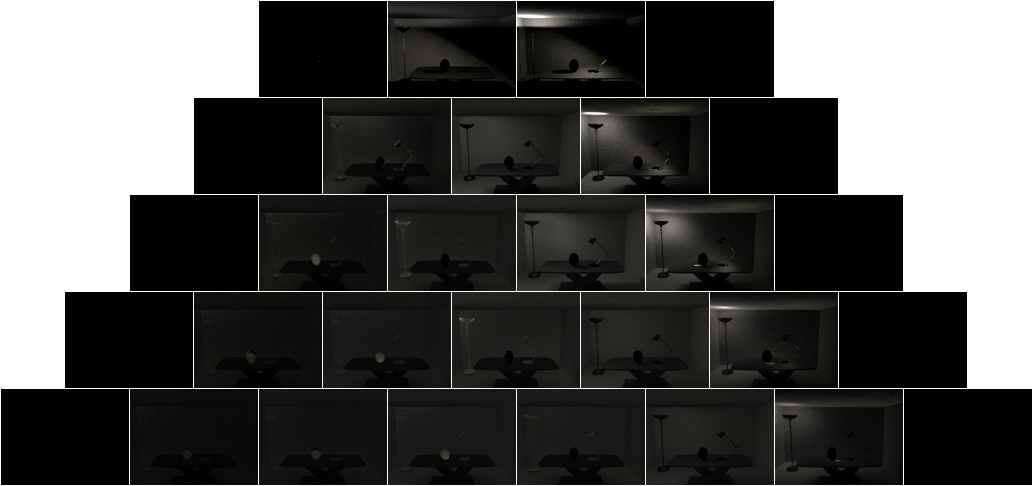
The above image show the length 4 strategies for specular bsdf + pinhole camera (from left \((s=0, t=4)\) to right \((s=4, t=0)\) ) Divide by 5 is definitely not enough to serve the purpose of combing length 4 strategies here.

Even we assume we won't encounter Dirac distribution, assign equal weight to each strategy doesn't provide the optimal result anyway. We see that certain strategy work particularly good on certain scenario, it doesn't make sense to add in other inferior strategy in this scenario to downgrade the result. The problem is: how we know which strategy work best on which scenario?

Veach95 introduced multiple importance sampling to solve this problem. The sampling combination techniques were applied to several rendering related topics includes: direct lighting sampling, final gathering, and bidirectional path tracing. Lafortune publish bidirectional path tracing around the same time with Veach, but the paper didn't formalize the way to combine different sampling strategies. My personal feeling is that bdpt become a powerful beast after applying multiple importance sampling. It was cool to come up result with multiple strategies, but determine which strategy is better in run time is mind-blowing cool :P

The multiple importance sampling estimator:

$$F=\sum_{i=1}^{n}\frac{1}{n_{i}}\sum_{j=1}^{n_{i}}\omega_{i}(X_{i,j})\frac{f(X_{i,j})}{pdf_{i}(X_{i,j})}$$

where \(n\) is the number of sampling techniques, and \(n_{i}\) is the number of sample for technique \(i\). With the power heuristic approach Veach propose:

$$\omega_{i} = (n_{i}pdf_{i}(X_{i,j}))^2/\sum_{k=1}^{n}(n_{k}pdf_{k}(X_{k,j}))^2$$

For example, we got a length 3 path come up with \((s=2,t=2)\) strategy, and we would like to have its MIS weight. What we need will be figure out the pdf to form this path with other strategies \(P_{A}(\bar{x}_{s=0, t=4})\), \(P_{A}(\bar{x}_{s=1, t=3})\),  \(P_{A}(\bar{x}_{s=3, t=1})\),  \(P_{A}(\bar{x}_{s=4, t=0})\) The \(n_{i}\) can simply be treated as 1 since we form every strategies for each integration samples. Expand the result:
$$\omega_{s=2,t=2}(\bar{x}) = \frac{P_{A}(\bar{x}_{s=2, t=2})^2}{P_{A}(\bar{x}_{s=0, t=4})^2 + P_{A}(\bar{x}_{s=1, t=3})^2+ P_{A}(\bar{x}_{s=2, t=2})^2+P_{A}(\bar{x}_{s=3, t=1})^2+P_{A}(\bar{x}_{s=4, t=0})^2}$$

Veach97 use the notation \(k=s+t-1\) and \(p_{i} = P_{A}(\bar{x}_{s=i, t=s+t-i})\), rewritten path \(\bar{x}_{s,t}\) as \(\bar{x} = x_{0}...x_{k}\). This simplify the power heuristic equation to \(\omega_{s,t} = \frac{p_{s}^{2}}{\sum_{i}p_{s}^{2}}\) . In above equation:
$$\omega_{s=2,t=2}(\bar{x}) = \frac{p_{2}^2}{p_{0}^2 + p_{1}^2+ p_{2}^2+p_{3}^2+p_{4}^2}$$
where:
\(p_{0} = P_{A}(x_{3})P_{\omega^{\perp}}(x_{3}\rightarrow x_{2})G(x_{2}\leftrightarrow x_{3})P_{\omega^{\perp}}(x_{2}\rightarrow x_{1})G(x_{1}\leftrightarrow x_{2})\)

\(\:\:\:\:\:\:\:\:\:P_{\omega^{\perp}}(x_{1}\rightarrow x_{0})G(x_{0}\leftrightarrow x_{1})\)

\(p_{1} = P_{A}(x_{3})P_{\omega^{\perp}}(x_{3}\rightarrow x_{2})G(x_{2}\leftrightarrow x_{3})P_{\omega^{\perp}}(x_{2}\rightarrow x_{1})G(x_{1}\leftrightarrow x_{2})P_A(x_{0})\)

\(p_{2} = P_{A}(x_{3})P_{\omega^{\perp}}(x_{3}\rightarrow x_{2})G(x_{2}\leftrightarrow x_{3})P_{\omega^{\perp}}(x_{0}\rightarrow x_{1})G(x_{0}\leftrightarrow x_{1})P_A(x_{0})\)

\(p_{3} = P_{A}(x_{3})P_{\omega^{\perp}}(x_{1}\rightarrow x_{2})G(x_{1}\leftrightarrow x_{2})P_{\omega^{\perp}}(x_{0}\rightarrow x_{1})G(x_{0}\leftrightarrow x_{1})P_A(x_{0})\)

\(p_{4} = P_{\omega^{\perp}}(x_{2}\rightarrow x_{3})G(x_{2}\leftrightarrow x_{3})P_{\omega^{\perp}}(x_{1}\rightarrow x_{2})G(x_{1}\leftrightarrow x_{2})\)

\(\:\:\:\:\:\:\:\:\:P_{\omega^{\perp}}(x_{0}\rightarrow x_{1})G(x_{0}\leftrightarrow x_{1})P_A(x_{0})\)

All ingredients (\(P_{\omega^\perp}\),  \(P_{A}\), \(G\)) can be collected during the path building stage. In fact, Veach even did a clever optimization to avoid duplicate computation between different \(p_{i}\):
$$\omega_{s,t} = \frac{p_{s}^{2}}{\sum_{i}p_{s}^{2}}=\frac{1}{\sum_{i}(p_{i}/p_{s})^{2}}$$

By treating the current \(p_{s}=1\), we can come up the other \(p_{i}\) related to \(p_{s}\) using the equation:

\(\frac{p_{1}}{p_{0}} = \frac{P_{A}(x_{0})}{P_{\omega^{\perp}}(x_{1} \rightarrow x_{0} )G(x_{1} \leftrightarrow x_{0})}\)

\(\frac{p_{i+1}}{p_{i}} = \frac{P_{\omega^{\perp}}(x_{i-1} \rightarrow x_{i}) G(x_{i-1} \leftrightarrow x_{i})}{P_{\omega^{\perp}}(x_{i+1} \rightarrow x_{i}) G(x_{i+1} \leftrightarrow x_{i})}\) for \( 0 < i < k \)

\(\frac{p_{k+1}}{p_{k}} = \frac{P_{\omega^{\perp}}(x_{k-1} \rightarrow x_{k}) G(x_{k-1} \leftrightarrow x_{k})}{P_{A}(x_{k})}\)

and on the reverse side:
\(\frac{p_{0}}{p_{1}} = \frac{P_{\omega^{\perp}}(x_{1} \rightarrow x_{0}) G(x_{1} \leftrightarrow x_{0})}{P_{A}(x_{0})}\)

\(\frac{p_{i-1}}{p_{i}} = \frac{P_{\omega^{\perp}}(x_{i} \rightarrow x_{i-1}) G(x_{i-1} \leftrightarrow x_{i})}{P_{\omega^{\perp}}(x_{i-2} \rightarrow x_{i-1}) G(x_{i-2} \leftrightarrow x_{i-1})}\) for \( 1 < i \leq k \)

\(\frac{p_{k}}{p_{k+1}} = \frac{P_{A}(x_{k})}{P_{\omega^{\perp}}(x_{k-1} \rightarrow x_{k}) G(x_{k-1} \leftrightarrow x_{k})}\)

There are......some devils hidden in the details that need special treatments.

First, while reusing the path by connecting different path vertex from light path and eye path, the end point pdf need to be reevaluate since the connection changes the outgoing direction:

Second, \(\frac{p_{k+1}}{p_{k}} = 0 \) when \(p_{k+1}\) is a camera with Dirac distribution (pinhole camera) since there are 0 chance you can hit a pinhole camera.

Third,  \(\frac{p_{0}}{p_{1}} = 0\) when \(p_{0}\) is a light with Dirac distribution (point light, spot light....etc) since there are 0 chance you can hit a point/spot light.

Fourth, when \(x_{j}\) stands for a surface point with specular bsdf, \(p_{j} = 0\) and \(p_{j+1} =0\) Veach97 contains a detail explanation of this exception handling in 10.3.5, the basic idea is, when \(p_{j} = 0\):

\(\frac {p_{j}}{p_{j-1}} = \frac{P_{\omega^{\perp}}(x_{j-2} \rightarrow x_{j-1}) G(x_{j-2} \leftrightarrow x_{j-1})}{P_{\omega^{\perp}}(x_{j} \rightarrow x_{j-1}) G(x_{j} \leftrightarrow x_{j-1})}\) contains a \(P_{\omega^{\perp}}(x_{j} \rightarrow x_{j-1}) \) in denominator which is a number that is not an actual pdf but a hack to get integration working, let's just call it evil alien number for now

\(\frac {p_{j}}{p_{j-1}}\frac {p_{j+1}}{p_{j}} =\frac{P_{\omega^{\perp}}(x_{j-2} \rightarrow x_{j-1}) G(x_{j-2} \leftrightarrow x_{j-1})}{P_{\omega^{\perp}}(x_{j} \rightarrow x_{j-1}) G(x_{j} \leftrightarrow x_{j-1})} \frac{P_{\omega^{\perp}}(x_{j-1} \rightarrow x_{j}) G(x_{j-1} \leftrightarrow x_{j})}{P_{\omega^{\perp}}(x_{j+1} \rightarrow x_{j}) G(x_{j} \leftrightarrow x_{j+1})}\) evil alien number still sticks in denominator :|

\(\frac {p_{j}}{p_{j-1}}\frac {p_{j+1}}{p_{j}}\frac {p_{j+2}}{p_{j+1}} =\frac{P_{\omega^{\perp}}(x_{j-2} \rightarrow x_{j-1}) G(x_{j-2} \leftrightarrow x_{j-1})}{P_{\omega^{\perp}}(x_{j} \rightarrow x_{j-1}) G(x_{j} \leftrightarrow x_{j-1})} \frac{P_{\omega^{\perp}}(x_{j-1} \rightarrow x_{j}) G(x_{j-1} \leftrightarrow x_{j})}{P_{\omega^{\perp}}(x_{j+1} \rightarrow x_{j}) G(x_{j} \leftrightarrow x_{j+1})}\frac{P_{\omega^{\perp}}(x_{j} \rightarrow x_{j+1}) G(x_{j} \leftrightarrow x_{j+1})}{P_{\omega^{\perp}}(x_{j+2} \rightarrow x_{j+1}) G(x_{j+2} \leftrightarrow x_{j+1})}\) 

The interesting thing happen, another evil alien number \(P_{\omega^{\perp}}(x_{j} \rightarrow x_{j+1})\) appears in the nominator. To make thing even more interesting, this two number are actually the same number that can cancel each other. Yes I questioned myself once whether this two number is the same number and the result is true. In pure specular reflection case (mirror) there are both 1. In reflection/transmission combine material like glass, depends on the implementation, it may be 0.5 (giving half half chance to do the transmission or reflection), it may be a \(F(\omega_{o}, \omega_{i})\) Fresnel number so that you can do a bit importance sampling for this bsdf. 0.5 is self explanatory enough that pdf from \(\omega_{o}\) to \(\omega_{i}\) is the same as  \(\omega_{i}\) to \(\omega_{o}\). Fresnel number if you examine the equation carefully, pdf from \(\omega_{o}\) to \(\omega_{i}\) is still the same as  \(\omega_{i}\) to \(\omega_{o}\) :) 

The conclusion: a specular surface point  \(x_{j}\)  will bring an evil alien number to pdf \(p_{j}\) and \(p_{j+1}\) that this two pdf shouldn't be counted in the final weighting calculation, but as long as we move on to  \(p_{j+2}\), everything goes back to normal.

With the above gotcha in mind, here is my implementation of multiple importance sampling weight evaluation:

And this is how the above first bounce strategies looks like after assign appropriate MIS weight:

You can see the high variance noise (estimator with low pdf) got smooth out and different strategies only preserve the estimator result that with high pdf. The most important thing is: the added on result, still converge correctly compare to the Mitsuba reference.

battle royale round 3: bdpt rendering vs path tracing Mitsuba reference

One thing to notice is that even this scene is not a particularly fun one, bdpt already show that it can use much less samples converging to similar result path tracing did (the above comparison, bdpt use 196 spp, Mitsuba reference uses 400 spp) Though the rendered images are kinda boring (cornell box all the way til the end :P ) The bidirectional path tracing is roughly complete now, and I have to say, OMG!......this journey is definitely not a piece of cake for myself. Time to open up a beer for a small celebration! In the next post, I would try to come up some relatively more interesting images and do a postmortem of this round of implementation.

Bidirectional Path Tracing 7 - Implement every s,t combination strategies

After implemented t=1 strategy light tracing and visually verify the result can converge to s=1 path tracing, I move on to implement t=0 strategy light tracing: shooting ray from light and bounce around the scene until it slams on camera lens. This is probably the worst strategy generally when lens is small compare to the scene since it has so little chance the sample can hit the lens. It can't even render anything if the camera is a pinhole model since ray will never intersect a infinitely small camera lens (just like s=0 strategy never works when the bouncing ray try to intersect a point light) But we are going to implement every strategy anyway, so I would like to prove this strategy can converge (when there are enough amount of samples) to correct result.

One small new things to add is that I need to implement disk geometry to simulate camera lens (you didn't implement disk geometry!? @@  yup....I live in the sphere and polygon mesh world for quite some while) so that ray can hit it. It was a small quadric exercise and there it is:

One good thing for t=0 strategy is that you don't need to implement shadow ray testing since you never connect light pah with eye path. The code logic looks simpler and each sample is cheaper to evaluate as the result, still....it is really really slow to converge compare to t=1 light tracing and s=1 path tracing....reallllllly sloooooooow!

This is how it looks like in a simple dof scene with 100 samples

Crank it up to 10000 samples per pixel, still noisy....

The Mitsuba right side path tracing reference uses around 200 spp

Two strategies work, now move to implement all different strategies, which is the first 50% of bidirectional path tracing. The rough idea is: we create a path from light, we create a path from camera, we connect every end points of light path and camera path to form paths with different strategies and evaluate the unweighted contribution \(C_{s,t}^{*}\) . For example, to render a 2 bounces render, we need to integrate paths with maximum length 4. We generate a length 4 path from light, we generate a length 4 path from camera, and we can connect the end points of two paths to form the following strategies:

length 1 : (s=2, t=0), (s=1, t=1), (s=0, t=2) direct visible light

length 2 : (s=3, t=0), (s=2, t=1), (s=1, t=2), (s=0, t=3) direct lighting

length 3 : (s=4, t=0), (s=3, t=1), (s=2, t=2), (s=1, t=3), (s=0, t=4) 1st bounce lighting

length 4 : (s=5, t=0), (s=4, t=1), (s=3, t=2), (s=2, t=3), (s=1, t=4), (s=0, t=5) 2nd bounce lighting

It's a bit of waste but I do throw away the combination that is longer than the specified max path length. I feel this makes the code logic looks cleaner and rendering behavior more consistent (there won't be path length 5 result added into render when specified max length 4 in this implementation) Since there can be multiple strategies to generate a path, simply added all the strategies to the final render image will result to a over blown image. The first draft of implementation add mDebugS, mDebugT flags to specify which s, t to be added into the final rendering. This is actually a good debug resource since I can specify a particular light path to render and isolate down whether the bug only happen in specific path. The implementation of eval contribution for every s, t combination is wrapped in BDPT::evalContribution:

The constructEyePath and constructLightPath are really similar that I just list one of them in the following code segments. In the beginning I was planning to wrap this two as one utility function but the slight difference stops me to do that in the first try, maybe it should be refactored to one in the long rung:

and here are some images only display 1st bounce lighting for debug purpose during the development:

s=1, t=3 first bounce for glossy material

s=2, t=2 first bounce for glossy material

s=3, t=1 first bounce for glossy material

the above debug images will converge when we cranked up the sample number, but even in this simple setup we can tell different strategy have different converge speed compare to other strategies. In the above images, s=1,t=3 path tracing strategy seems to be the better strategy compare to the other two. How we determine which strategy is good for which scenario, and which strategy is better for other scenario? This is where multiple importance sampling come to rescue :) and I'll try to talk about my interpretation in the next post.

Bidirectional Path Tracing 6 - Implement light tracing

Like path tracing have s = 0 (trace ray from camera til it hits the light) and s = 1 (trace ray from camera, connect the ray intersection with a light sample) strategies, light tracing also have t = 0 (trace ray from light til it hits the lens) and t = 1 (trace ray from light, connect the ray intersecgtion with a camera lens sample) strategies. My first light tracing implementation was t = 1 strategy, mainly because it can handle edgy case that t = 0 strategy can't handle, ie, pinhole camera. (you can't hit a point light if you use s = 0 strategy right? ;P ) Also, when the lens is a really small object in the scene, it is way easier to connect a sample from the lens then try to hit the lens, which means, the t = 1 strategy generally converge faster than the t = 0 strategy.

The implementation is really straightforward once we have the \(C_{s,t}^{*}\) equation in the previous post. We set up a max path length (the level of bounces, 2 for only direct lighting, 3 for one bounce, 4 for two bounces....etc) then we evaluate \(C_{1,1}^{*}\), \(C_{2,1}^{*}\), \(C_{3,1}^{*}\), \(C_{4,1}^{*}\) ...... I tried to match the code variables as close as the original equation, but I do made an extra branch statement to deal with the \(L_{e}^{(0)}\), \(L_{e}^{(1)}\), \(f_{s}(y_{-1} \rightarrow y_{0}\rightarrow y_{1})\) case mentioned in previous post. The guts and bone of light tracing is wrapped in LightTracer::splatFilmT1 and it looks like this:

at the end of the render, we output image with the unbiased filter estimator described in previous post

We got light tracing implemented, and here comes the scary question: is the result correct? This small toy previous implemented Whitted style ray tracing, unidirectional path tracing, ambient occlusion, they all look different for sure, but theoretically, light tracing should converge to the same result as path tracing :| How do I know whether my light tracing is correct? or, how do I even know whether my path tracing is correct?

This was actually a question colleague asked me before I started working on bdpt, and the suggestion he made was: use the mighty Mitsuba for comparison. Face to face, fist to fist. as he suggested, I spent some times to build a Mitsuba scene that is 100% matching a simple personal scene with personal scene description format (manual conditioning...that kinda reminds me some not that pleasant tasks I've worked on before as a daily job...) and close my eye....finger crossed....hit enter!

the Mitsuba reference

The good news is... the path tracing implementation is identical to Mitsuba at the first hit (in this simplest setting...I have no confidence whether it works if I throw in volume and some other sexy bsdf yet :P ) whew!

the bloody face to face battle royale

The light tracing...as my memory served, didn't get that luck. The debug process was not pretty fun, but at least I isolate down it's light tracing having problem instead of the whole renderer having problem thanks to the existing reference. The bugs I remembered including: the wrong filter normalization, the wrong order of \(\omega_{o}\), \(\omega_{i}\) , and the purest evil: I didn't reset the tfar after ray intersect something: this bug made the direct lighting looks identical but problem occurs after the first bounce, and it took me probably 3 days to find it.... :| Enough of complaints, after fixing this bug fixing that bug, light tracing also went to the same converge result at the end. Hooray~~

light trace vs path trace, battle royale round 2

Personally I feel implementing light tracing marks half way through the bidirectional path tracing. We prove the symmetry indeed exist (with human eyes....) The next thing we are going to do is implementing all the s, t combination strategies and make sure they converges, after that... it will be the final boss (which is the most powerful feature for bidirectional path tracing in my opinion): combine all the strategy through multiple importance sampling!

Bidirectional Path Tracing 5 - More than one way to form a path

Plug in the area space light transport equation:

$$L( x'\to x'' )=L_{e}( x'\to x')+\int_{A }L_{i}( x \to x' )f_{s}(x \to x' \to x'')G(x \leftrightarrow  x')dx $$

into the measurement equation:

$$I = \int_{A_{lens}} \int_{A_{film}} W_{e}(x_{film}\rightarrow  x_{lens})L(x_{film}\rightarrow  x_{lens}) G(x_{film}\leftrightarrow  x_{lens}) dx_{film} dx_{lens}$$

recursive expand it, we get:

\(I = \sum_{k=1}^{\infty}\int_{A^{k+1}}L_{e}(x_{0}\rightarrow x_{1})G(x_{0}\leftrightarrow x_{1})\prod_{i=1}^{k-1}f_{s}(x_{i-1} \rightarrow x_{i} \rightarrow x_{i+1})G(x_{i} \leftrightarrow x_{i+1})\)

\(\:\:\:\:\:\:\:\:W_{e}(x_{k-1} \rightarrow x_{k}) dA(x_{0})...dA(x_{k}) \)

\(= \int_{A^{2}}L_{e}(x_{0}\rightarrow x_{1})G(x_{0}\leftrightarrow x_{1})W_{e}(x_{0} \rightarrow x_{1})dA(x_{0})dA(x_{1})\)

\(+ \int_{A^{3}}L_{e}(x_{0}\rightarrow x_{1})G(x_{0}\leftrightarrow x_{1})f_{s}(x_{0} \rightarrow x_{1} \rightarrow x_{2})G(x_{1}\leftrightarrow x_{2})\)

\(\:\:\:\:\:\:\:\:W_{e}(x_{1} \rightarrow x_{2})dA(x_{0})dA(x_{1})dA(x_{2})\)

\(+ \int_{A^{4}}L_{e}(x_{0}\rightarrow x_{1})G(x_{0}\leftrightarrow x_{1})f_{s}(x_{0} \rightarrow x_{1} \rightarrow x_{2})G(x_{1}\leftrightarrow x_{2})f_{s}(x_{1} \rightarrow x_{2} \rightarrow x_{3})\)

\(\:\:\:\:\:\:\:\:G(x_{2}\leftrightarrow x_{3})W_{e}(x_{2} \rightarrow x_{3})dA(x_{0})dA(x_{1})dA(x_{2})dA(x_{3})\)

\(+\:\: ............\)

In English:

measurement result (radiance)

= integrate all measured value with path length 1 to path length infinity

= integrated path length 1 measured value ( direct visible light)

+ integrated path length 2 measured value ( direct lighting )

+ integrated path length 3 measured value ( first bounce lighting )

+ ....

All these paths can be built by tracing ray from camera or from light, or from both and connect together, there are many (be more specific, n + 1 methods if the path contains n vertices) ways to form a path. We can pick out a length 3 (first bounce, 4 vertices) path \(x_{0}x_{1}x_{2}x_{3}\)as case study (for all different lengths it's still the same thing, just feel length 3 is on a sweet spot to cover the idea). Follow Veach's naming convention, \(s\) stands for the path vertices start tracing from light, \(t\) stands for the path vertices start tracing from camera (or eye). For path length 3, s + t = 4, we have 5 kinds of ways to form the path:

\(s = 0, t = 4\)  trace ray from camera until it hits the light (naive path tracing)

\(s = 1, t = 3\)  trace ray from camera and connect to a sample on light (commonly used path tracing)

\(s = 2, t = 2\)  trace ray from both light and camera, connect them together
\(s = 3, t = 1\)  trace ray from light and connect to a sample on camera lens ( t = 1 style light tracing )

\(s = 4, t = 0\)  trace ray from light until it hits the camera lens (t = 0 style light tracing )

The function to be integrated for path \(x_{0}x_{1}x_{2}x_{3}\) is the same for any s, t combinations:

\(f(\bar{x}) = L_{e}(x_{0}\rightarrow x_{1})G(x_{0}\leftrightarrow x_{1})f_{s}(x_{0} \rightarrow x_{1} \rightarrow x_{2})G(x_{1}\leftrightarrow x_{2})f_{s}(x_{1} \rightarrow x_{2} \rightarrow x_{3})\)

\(\:\:\:\:\:\:\:\:G(x_{2}\leftrightarrow x_{3})W_{e}(x_{2} \rightarrow x_{3})\)

The pdf to form the path is different from one combination to another combination though. In Veach97 the pdf usually measured in "projection solid angle" space. It is defined as:

$$pdf_{\omega^{\perp}}(x, \omega) = pdf_{\omega}(x, \omega) / \cos\theta$$

and since we can transform pdf from solid angle space to area space as:

$$pdf_{A}(x, {x}') = pdf_{\omega}(x, \omega)\cos\theta_{{x}'}/d(x\leftrightarrow{x}')^{2}$$

The introduction of projection solid angle brings the geometry term \(G\) into battle:

$$pdf_{A}(x, {x}') = pdf_{\omega^{\perp}}(x, \omega)G(x\leftrightarrow{x}')$$

With this projection solid angle \(pdf_{\omega^{\perp}}\), the \(pdf_{A}\) for different s, t combination can be written as:

\(pdf_{A}(\bar{x}_{s=0,t=4}) =pdf_{A}(x_{3})pdf_{\omega^{\perp}}(x_{3}\rightarrow x_{2})G(x_{2}\leftrightarrow x_{3}) pdf_{\omega^{\perp}}(x_{2}\rightarrow x_{1})G(x_{1}\leftrightarrow x_{2})\)

\(\:\:\:\:\:\:\:\:pdf_{\omega^{\perp}}(x_{1}\rightarrow x_{0})G(x_{0}\leftrightarrow x_{1})\)

\(pdf_{A}(\bar{x}_{s=1,t=3}) =pdf_{A}(x_{3})pdf_{\omega^{\perp}}(x_{3}\rightarrow x_{2})G(x_{2}\leftrightarrow x_{3}) pdf_{\omega^{\perp}}(x_{2}\rightarrow x_{1})G(x_{1}\leftrightarrow x_{2})\)

\(\:\:\:\:\:\:\:\:pdf_{A}(x_{0})\)

\(pdf_{A}(\bar{x}_{s=2,t=2}) =pdf_{A}(x_{3})pdf_{\omega^{\perp}}(x_{3}\rightarrow x_{2})G(x_{2}\leftrightarrow x_{3}) pdf_{\omega^{\perp}}(x_{1}\leftarrow x_{0})G(x_{0}\leftrightarrow x_{1})\)

\(\:\:\:\:\:\:\:\:pdf_{A}(x_{0})\)

\(pdf_{A}(\bar{x}_{s=3,t=1}) =pdf_{A}(x_{3})pdf_{\omega^{\perp}}(x_{2}\leftarrow x_{1})G(x_{1}\leftrightarrow x_{2}) pdf_{\omega^{\perp}}(x_{1}\leftarrow x_{0})G(x_{0}\leftrightarrow x_{1})\)

\(\:\:\:\:\:\:\:\:pdf_{A}(x_{0})\)

\(pdf_{A}(\bar{x}_{s=4,t=0}) =pdf_{\omega^{\perp}}(x_{3}\leftarrow x_{2})G(x_{2}\leftrightarrow x_{3})pdf_{\omega^{\perp}}(x_{2}\leftarrow x_{1})G(x_{1}\leftrightarrow x_{2}) \)

\(\:\:\:\:\:\:\:\:pdf_{\omega^{\perp}}(x_{1}\leftarrow x_{0})G(x_{0}\leftrightarrow x_{1})pdf_{A}(x_{0})\)

Divide \(f(\bar{x})\) by \(pdf_A\), we got five different Monte Carlo estimators \(C_{s,t}^{*}\)for path  \(x_{0}x_{1}x_{2}x_{3}\):

\(C_{0,4}^{*} =\frac{ L_{e}(x_{0}\rightarrow x_{1})f_{s}(x_{0} \rightarrow x_{1} \rightarrow x_{2})f_{s}(x_{1} \rightarrow x_{2} \rightarrow x_{3})W_{e}(x_{2} \rightarrow x_{3}) }{pdf_{A}(x_{3})pdf_{\omega^{\perp}}(x_{3}\rightarrow x_{2})pdf_{\omega^{\perp}}(x_{2}\rightarrow x_{1})pdf_{\omega^{\perp}}(x_{1}\rightarrow x_{0})}\)

\(C_{1,3}^{*} =\frac{ L_{e}(x_{0}\rightarrow x_{1})G(x_{0}\leftrightarrow x_{1})f_{s}(x_{0} \rightarrow x_{1} \rightarrow x_{2})f_{s}(x_{1} \rightarrow x_{2} \rightarrow x_{3})W_{e}(x_{2} \rightarrow x_{3}) }{pdf_{A}(x_{3})pdf_{\omega^{\perp}}(x_{3}\rightarrow x_{2}) pdf_{\omega^{\perp}}(x_{2}\rightarrow x_{1})pdf_{A}(x_{0})}\)

\(C_{2,2}^{*} =\frac{ L_{e}(x_{0}\rightarrow x_{1})f_{s}(x_{0} \rightarrow x_{1} \rightarrow x_{2})G(x_{1}\leftrightarrow x_{2})f_{s}(x_{1} \rightarrow x_{2} \rightarrow x_{3})W_{e}(x_{2} \rightarrow x_{3}) }{pdf_{A}(x_{3})pdf_{\omega^{\perp}}(x_{3}\rightarrow x_{2}) pdf_{\omega^{\perp}}(x_{1}\leftarrow x_{0})pdf_{A}(x_{0})}\)

\(C_{3,1}^{*} =\frac{ L_{e}(x_{0}\rightarrow x_{1})f_{s}(x_{0} \rightarrow x_{1} \rightarrow x_{2})f_{s}(x_{1} \rightarrow x_{2} \rightarrow x_{3})G(x_{2}\leftrightarrow x_{3})W_{e}(x_{2} \rightarrow x_{3}) }{pdf_{A}(x_{3})pdf_{\omega^{\perp}}(x_{2}\leftarrow x_{1}) pdf_{\omega^{\perp}}(x_{1}\leftarrow x_{0})pdf_{A}(x_{0})}\)

\(C_{4,0}^{*} =\frac{ L_{e}(x_{0}\rightarrow x_{1})f_{s}(x_{0} \rightarrow x_{1} \rightarrow x_{2})f_{s}(x_{1} \rightarrow x_{2} \rightarrow x_{3})W_{e}(x_{2} \rightarrow x_{3}) }{pdf_{\omega^{\perp}}(x_{3}\leftarrow x_{2})pdf_{\omega^{\perp}}(x_{2}\leftarrow x_{1}) pdf_{\omega^{\perp}}(x_{1}\leftarrow x_{0})pdf_{A}(x_{0})}\)

all geometry terms got cancelled out except the one that connect end points between light path and eye path. The 5 estimators show beautiful symmetry between each opposite side (s1t3 vs s3t1, s0t4 vs s4t0 ). In fact, Veach made all path length cases into a generalized equation and it is one of the largest building block for bidirectional path tracing:

For a path \(\bar{x}_{s,t} = y_{0}...y_{s-1}z_{t-1}...z_{0}\), the unweighted contribution can be computed as \(C_{s,t}^{*} = \alpha_{s}^{L}c_{s,t}\alpha_{t}^{E}\), where light path factor:

\(\alpha_{0}^{L} = 1\)

\(\alpha_{1}^{L} = L_{e}^{(0)}(y_{0}) / P_{A}(y_{0})\)

\(\alpha_{i}^{L} = \frac{f_{s}(y_{i-3} \rightarrow y_{i-2} \rightarrow y_{i-1})}{P_{\omega^{\perp}}(y_{i-2} \rightarrow y_{i-1})} \alpha_{i-1}^{L}\) for \(i \geq 2\)

and eye path factor:

\(\alpha_{0}^{E} = 1\)

\(\alpha_{1}^{E} = W_{e}^{(0)}(z_{0}) / P_{A}(z_{0})\)

\(\alpha_{i}^{E} = \frac{f_{s}(z_{i-3} \rightarrow z_{i-2} \rightarrow z_{i-1})}{P_{\omega^{\perp}}(z_{i-2} \rightarrow z_{i-1})} \alpha_{i-1}^{E}\) for \(i \geq 2\)

and connection factor:

\(c_{0,t} = L_{e}(z_{t-1} \rightarrow z_{t-2})\)

\(c_{s,0} = W_{e}(y_{s-2} \rightarrow y_{s-1})\)

\(c_{s,t} = f_{s}(y_{s-2} \rightarrow y_{s-1} \rightarrow z_{t-1})G(y_{s-1} \leftrightarrow z_{t-1}) f_{s}(y_{s-1} \rightarrow z_{t-1} \rightarrow  \rightarrow z_{t-2} ) \) for \(s, t > 0\)

One notation looks a bit weird is that \(L_{e}^{(0)}\) and \(W_{e}^{(0)}\). Veach97 call this "spatial component" and define the radiance/importance as:

\(L_{e}(y_{0} \rightarrow y_{1}) = L_{e}^{(0)}(y_{0})L_{e}^{(1)}(y_{0} \rightarrow y_{1})\)

\(W_{e}(z_{1} \rightarrow z_{0}) = W_{e}^{(0)}(z_{0})W_{e}^{(1)}(z_{1} \rightarrow z_{0})\)

\(f_{s}(y_{-1} \rightarrow y_{0} \rightarrow y_{1}) =  L_{e}^{(1)}(y_{0} \rightarrow y_{1})\)

\(f_{s}(z_{1} \rightarrow z_{0} \rightarrow z_{-1}) =  W_{e}^{(1)}(z_{1} \rightarrow z_{0})\)

The purpose of this notation, according to Veach, is to reduce the number of special cases that need to be considered, by interpreting the directional component of emission as a BSDF. Though personally, I don't feel this particular tempting to me. Writing a branch VS writing another bsdf interface for light and camera, I prefer a branch.

My fingers are aching by typing latex equation now and it's kinda dry to go through the math, but at this point we have all the stuff I need to implement light tracing : importance, filter, path contribution \(C_{s,t}^{*}\). The next post will focus on the light tracing implementation, and some (not that academic) ways to verify the result. 

Bidirectional Path Tracing 4 - A tweak of the filter

In Veach97 10.3.1 each pixel value \(I_{j}\) in the image is defined as a weighted average

$$I_{j} = \int\int_{D}h_{j}(u, v)I(u, v)dudv$$

where \(D\) is the image region (in world space, not pixel space), and \(h_{j}\) is the filter function (for example, a 2x2 box filter) for pixel j. When the filter function satisfies the criteria that \(\int\int_{D}h_{j}(u, v)dudv=1\), we filtered the measurement equation integration result \(I\) across lens and film area to one particular pixel \(I_{j}\) . This is a bit counter intuitive for me at the beginning: The measurement equation measure up a value related to the whole lens and film, and pixel value (what image rendering is actually looking for) is a post process product from the measurement value (by multiply importance \(W_{e}(x, \omega)\) and filter \(h_{j}(u, v)\) ) .

Since measurement equation contains integration across the whole film ( the \(D\) region), the samples we cast should be thrown across the whole film (For example, a 640x480 image with 4 samples per pixel, we throw out 640x480x4 samples to get the image value for pixel (123, 456). It doesn't sound make sense at first, but thinking further, all the other samples that pixel (123, 456) doesn't take get accumulated to other pixels, so we are not doing wasted work after all) The estimator for this equation would then be:

$$E(I_{j}) = 1/N \sum_{i=1}^{N}h_{j}(u_{i}, v_{i})I(u_{i}, v_{i}) / pdf_{A_{film}}(u_{i}, v_{i}) = D/N \sum_{i=1}^{N}h_{j}(u_{i}, v_{i})I(u_{i}, v_{i}) $$

In the path tracing world that shooting ray from camera, we usually know which samples will contribute to a certain pixel (continue the 2x2 box filter example, the final (123, 456) pixel value would only be affect by the ray shooting across range (122, 455)-&gt;(124, 457) ) &nbsp;In fact, the filter equation usually used for path tracing looks like:

$$E(I_{j}) = \frac{\sum_{i=1}^{N}h_{j}(u_{i}, v_{i})I(u_{i}, v_{i})}{\sum_{i=1}^{N}h_{j}(u_{i}, v_{i})}$$

The coding logic is roughly like: for each sample we got a radiance value, we add value \(h_{j}(u_{i}, v_{i})I(u_{i}, v_{i})\) across region this sample centered kernel can cover to the covered pixels, and add \(h_{j}(u_{i}, v_{i})\) to a separate weight value associated to that pixel. At the end, we normalize each pixel with their associated weight. This works for camera based tracing method since, again, we know which samples would contribute to which pixel. This doesn't work for light tracing method since, for each ray shoot out from light, we don't know which pixel it will slam on film after bouncing around the scene.

As a result, Veach97 10.3.4.3 propose that using equation \(E(I_{j}) = \frac{\sum_{i=1}^{N}h_{j}(u_{i}, v_{i})I(u_{i}, v_{i})}{ \sum_{i=1}^{N}h_{j}(u_{i}, v_{i})}\) for path tracing method, and use \(E(I_{j})= D/N \sum_{i=1}^{N}h_{j}(u_{i}, v_{i})I(u_{i}, v_{i})\) for light tracing method. That is, for light tracing method, we throw out total N samples, whenever a sample hit the film and lens, we added the sample contribution \(h_{j}(u_{i}, v_{i})I(u_{i}, v_{i})\) to nearby affected pixels. At the end, we multiply the whole image film by factor \(D/N\) where \(D\) is the film area in world space.

My previous filtering implementation use the path tracing method above, and there is one missing puzzle that need to be filled to get the light tracing method work: \(\int\int_{D}h_{j}(u, v)dudv=1\) . The filter was not normalized to film world area space, for example, again the 2x2 box filter, \(h_{j}(u_{i}, v_{i}) = 1 \) if \((u_{i}, v_{i})\) is in the 2x2 kernel range else 0, the integration result for this filter would be 2x2 = 4 pixel area. To normalize this box filter, \(h_{j}(u_{i}, v_{i}) \) need to be divide by 4 pixel area so the final kernel integration become 1. I added a virtual method getNormalizedTerm for all filters to query kernel integration result in pixel space, and during the adding sample to final image space, I add in one more divide by pixel area step to normalize pixel space integration to world space. The reason I didn't put thing together is that I don't want the filter functionality depends on film size (which should able to change its size without worrying about what filter it's paired to) So here we go, the getNormalizedTerm :


And the related film constructor/addSample changes:

One thing that I feel a bit awkward is that it's actually not a easy thing to integrate Gaussian filter in finite range (surprise! consider how beautiful it converge when integrate to infinity) that turns out I use a clumsy numerical approximation to get an approximated integration result. It's not really beautiful, but it serves the purpose ;)

In the next post I would like to write down the thoughts while looking in Veach97 10.2 : the ways to form a path, and its contribution to the final measurement (which is the \alpha weight I briefly mentioned in previous post ) It will be the ground work to start writing light tracing, and push it further to bidirectional path tracing.

Bidirectional Path Tracing 3 - Importance and measurement equation

The equation that integrate the power flow through focal lens and land on camera lens looks like this:
$$\Phi = \int_{A_{lens}} \int_{\Omega} L(x, \omega_{i}) cos\theta d\omega dx$$
We got the power, but we actually want the average radiance value in specific pixel (so that we can form the image, which is what ray tracing usually looking for). Is there any way that we can convert this power to radiance? Yes :) In Veach97 the equation actually has another extra term, and the equation does not explicitly integrate out power as result. It looks like this:
$$I = \int_{A_{lens}} \int_{\Omega} W_{e}(x, \omega)L(x, \omega_{i}) cos\theta d\omega dx$$
The original paper name this "measurement equation" and that extra term \(W_{e}(x, \omega)\) is named as importance. Measurement equation try to measure certain value related to power, and importance convert the power to that value. The following description is directly copied from Veach Chapter 4.5 (p115):

"For real sensors, \(W_{e}\) is called the flux responsivity of the sensor. The responding units are \(S/Watt\) (Watt is the unit for power), where \(S\) is the unit of sensor response. Depending on the sensor, \(S\) could represent a voltage, current, change in photographic film density, deflection of a meter needle, etc."

Ya that's how scientists write paper...they view problem in a broader term, try to solve voltage, current, change in photographic film density.....all in one equation....but wait! I just want the average radiance in particular pixel! Can you please just give me the \(W_{e}(x, \omega)\) for that?

It sounds silly now but this question is probably the one that trouble me longest while looking in the paper :| , and I think it's worthy to write it down as memo.

Start with measurement equation above:
\(I = \int_{A_{lens}} \int_{\Omega} W_{e}(x, \omega)L(x, \omega_{i}) cos\theta d\omega dx\)
We can transform the \(\Omega\) part solid angle integration to area space integration over the film area with an additional geometry term \(G\)  (like what we did in previous post):
\(I = \int_{A_{lens}} \int_{A_{film}} W_{e}(x_{film}\rightarrow  x_{lens})L(x_{film}\rightarrow  x_{lens}) G(x_{film}\leftrightarrow  x_{lens}) dx_{film} dx_{lens}\)

The \(A_{film}\) term is the world area of film. Again, we use the non real world CG camera model that film stands in front of lens (instead of behind lens like real world camera) and in the focus distance. That is, we treat the focus plane as film like the following image illustrates:

The Monte Carlo estimator for the area space equation looks like:
\(E(I)=\frac{1}{N}\sum_{i= 1}^{N}\frac{W_{e}(x_{film_{i}}\rightarrow  x_{lens_{i}})L(x_{film_{i}}\rightarrow  x_{lens_{i}}) G(x_{film_{i}}\leftrightarrow  x_{lens_{i}})}{pdf_{A}(x_{film_{i}})pdf_{A}(x_{lens_{i}})}\)
We want the \(W_{e}(x_{film_{i}}\rightarrow  x_{lens_{i}})\) term can transfer this measurement result to be radiance \(L(x_{film_{i}}\rightarrow  x_{lens_{i}})\), which gives us the result:
\(W_{e}(x_{film}\rightarrow  x_{lens})=\frac{pdf_{A}(x_{film})pdf_{A}(x_{lens})}{G(x_{film}\leftrightarrow  x_{lens})} = \frac{d(x_{film}\leftrightarrow  x_{lens})^{2}}{A_{film}A_{lens}cos\theta^{2}}\)
If we look in further to the above equation, \(A_{film}\) is proportional to \(d(x_{film}\leftrightarrow  x_{lens})^{2}\), which means distance is not a factor that would affect the result and we can use \(W_{e}(x_{film}\rightarrow  x_{lens})\) directly for \(W_{e}(x, \omega)\) where \(\omega\) is the shooting ray direction from \(x_{lens}\) to \(x_{film}\)

and now we can write some codes :)
A beautiful symmetry between radiance and importance is shaping up once we have importance in hand:
the image can be rendered through camera shooting rays generated by uniformly sampling camera lens and camera film, capturing incoming radiance through the ray and accumulate it to corresponding pixel. At the end, divide accumulated radiance by sample per pixel. This is the parh tracing style (in its simplest form).

the image can also be rendered through lights shooting rays generated by uniformly sampling light surface and hemisphere outgoing directions, capturing incoming importance through the ray, add light ray carrying weight (this weight value \(\alpha\) will be discussed in later post) multiplied importance to pixel corresponding to the incoming importance. At the end, divided accumulated radiance by total number of samples shoot out from light. This method is usually named as light tracing or particle tracing (I use the former naming since particle tracing short as pt is a bit confusing when mention it together with path tracing)

This two methods should converge to the same expectation value when sample numbers crank up (mathematically and theoretically :) we gonna write the light tracer to prove this by our eye! ) I got to say I was mind blown when I learn this symmetry, it's so Zen that kinda like that ancient Chinese philosopher talk ("Now I do not know whether I was then a man dreaming I was a butterfly, or whether I am now a butterfly, dreaming I am a man." - Zhuangzi)

The above method work as it is when each sample only contribute to one pixel (for example, sample (320.4, 510.6) only contributes radiance (320, 511), sample (128.7, 426.3) only contributes radiance (129, 426)), but that's not the case when we have filter kernel that would potentially contribute to multiple pixels per sample...(a simplest example, 2X2 box filter can contribute radiance to 4 pixels per sample), does the "divide by \(N\)(total number of samples shoot out from light)" still works for light tracing when filter jump in? Nope! we need to do some surgery work on filter if we want to get unbiased result, and we will talk about it in the next post :)

Bidirectional Path Tracing 2 - From solid angle space to area space

The rendering equation usually looks like this:
$$L( x,\vec{\omega _{o}} )=L_{e}(x, \vec{\omega _{o}})+\int_{\Omega }L_{i}( x_{i},\vec{\omega _{i}} )f_{s}(  x,\vec{\omega _{i}}, \vec{\omega _{o}} )cos \theta d\omega $$
We integrate the incoming radiance over hemisphere with BSDF, plus the emitted radiance and we get the result. The integration is in solid angle domain, therefore when we do the monte carlo estimator, our pdf is in solid angle domain: whether the pdf of sampling bsdf, or the pdf of sampling light (actually we usually sampling area lights in pdf with respect to area domain and then convert it to solid angle domain using equation: \(pdf\omega = pdfA/(cos \theta /d^{2})\) where \(d\) is the distance between intersection point to light surface sample point and  \(\theta\) is the angle between light surface normal and the direction from light surface sampled point to intersection.) The solid angle integration is roughly looks like this:

One of the mindset shifting while reading the paper for me was moving the integration from solid angle domain to area domain. That is: instead of shooting bounce rays around the solid angle hemisphere, we integrate the radiance coming from all the "surfaces in the scene". Replace the \(d\omega\) in solid angle integration with \( cos(\theta_{o}) / r^{2} dx\) in area domain, we see the equation become something like:
$$L( x'\to x'' )=L_{e}( x'\to x')+\int_{A }L_{i}( x \to x' )f_{s}(x \to x' \to x'')G(x \leftrightarrow  x')dx $$
where \(G(x \leftrightarrow  x') = V(x \leftrightarrow  x')\mid cos(\theta_{o})cos( \theta_{i'})\mid/\parallel x - x' \parallel^{2}\) (\(V\) stands for visibility test, aka occlusion test, aka shooting a shadow ray and make sure two point is visible to each other) Veach called this "The three-point form of the transport equations" (see Veach97 8.1) and the \(G\) is usually referred as the "geometry term". The illustration above can be transformed to area domain integration like this:

We are still trying to figure out the radiance \(Lo\) but the integration style is different, the final result value should be the same, ie. two different sampling methods should converge to same result at the end.

With above LTE to compute radiance, we further integrate radiance over the camera lens area and the solid angle extended by focal plane, and then we get the power flow through focal plane and land on camera lens (well in real life focal(film) plane should be behind the camera lens, but this is a commonly used CG approximation model and it made this integration easier to understand)

$$\Phi = \int_{A_{lens}} \int_{\Omega} L(x, \omega_{i}) cos\theta d\omega dx$$

And interesting stuff happened...LTE is a recursive equation (both left side and right side contains unknown value L) If we break it down by recursion levels, the power integration above can be think about as the combination of: integration of all the possible length 1 paths (2 vertices, one on lens, one on light) + integration of all the possible length 2 paths (3 vertices, one on lens, one on scene surfaces, one on light) + integration of all the possible length 3 paths (4 vertices, one on lens, two on scene surfaces, one on light).....+ integration of all possible length \(\infty\) paths...illustrated in the following images:

The cool thing is: there is no necessary order dependency between the area space integration! you can sample p3 and then sample p2, it doesn't matter, it's always "sample a surface point in the scene".  In solid angle space, that is, unidirectional path tracing, we always find the first intersection and then propagate to the first bounce, then second bounce, then third bounce. In area space you just keep choosing the point on surface and connect them together, there are plenty of freedom on the way you choose from surface to form a list of vertex connection (a path), you can start from light and shoot out particle as ray, bounce around the scene....you can start from camera and shoot out viewing ray, bounce around the scene....you can do both, and then connect them together! This is actual one key idea for bidirectional path tracing: there are many ways to skin a cat, we can try them out(....and then figure out which is the best way)

Veach97 formalize this idea as math equations in chapter 8.2 "The path integral formulation". We construct the paths of length 1 to length \(\infty\), we use monte carlo to approximate the integration, and then we can figure out the power flow from scene through film to lens,

Uhh...ya that does sounds kinda cool, but....isn't ray tracing usually want the radiance on a specified pixel instead of this power flow? Can we transform this power flow to radiance? These questions marks pop through my mind while reading through this part, and it's another new concepts "importance \(W_{e}\)" and "measurement equation" come to rescue at last. :)

Bidirectional Path Tracing 1 - Kickoff

After attending SIGGRAPH last year, I was chatting with colleagues about those inspiring contents in the talks like  "The Path Tracing Revolution in the Movie Industry", "Physically Based Shading in Theory and Practice". It seems clear the whole industry is shifting toward path tracing at this moment, but there are still no conclusion about what is the best way to do this. ( It was fun to see WETA first stated that you shouldn't aim at certain algorithm to build the software architecture and sacrifice the future extensibility, then Disney immediately came up to say "we are actually doing exactly what you said that shouldn't do"). "We should keep up our learning speed, and try to catch up those integrators knowledges that are moving so fast nowadays" was our chatting conclusion that day.

In Pixar's Renderman Art and Science Fair, they mentioned that the latest version Renderman supports Vertex Connection Merging (vcm) and ready for production use. My barely minimum understanding about vcm is that it mixed bidirectional path tracing(bdpt) and progressive photon map(ppm) with multiple importance sampling, and able to efficiently render some particular tricky light transport path (SDS, specular->diffuse->specular especially) that is sometimes even impossible to render with unidirectional path tracing. To get a better idea of how exactly it works, I guess I should first get myself familiar with bdpt and ppm, which I thought about implement it in this side project for quite some while.

So here we go, I tried to read through that famous Veach 97 again (I tried it once before, and got pretty confused about several key details...). After consuming quite some amount of coffee in Starbucks, I think this time I understand it a bit deeper :) . Definitely still far from throughout understanding, but should be enough to implement bdpt. I got a working implementation few days ago, and thought I should write my thought process down as memo. There are some particular points I struggled for days to figure out and I would like to share the thoughts for discussion. The original paper try to explain the whole idea with a broader application view while all I want is crank out some tiny pixels. The thoughts here, as a result, are mainly my interpretation about translating those math equation into codes. Hopefully after I write down the following posts, I can pick up the thoughts quicker next time.

The steps of this bdpt implementation are roughly listed below:

1. the mindset shifting from original path tracing style solid angle space light transport equation (LTE) to area space

2. understanding the idea of impoartance, Its zen symmetry to radiance and most importantly: how to evaluate its value?

3. how filter works in the bdpt world, and how to modify existing filter implementation to adapt and keep it backward compatible to the previous path tracing implementation

4. break down the unweighted contribution equation in Veach97 10.2

5. implement light tracing technique, which is actually more intuitive as high level idea than path tracing to me (shooting particle from light instead of shooting sensor ray from camera), and make sure the result is correct compare to the path tracing method

6. implement bdpt that can choose around different light/camera path (s, t) combination techniques

7. implement multiple importance sampling(MIS) to weight sum different s, t techniques

8. handle specular special case (I like point light and glass surface, until I need to deal them as exceptional case)

The reference:

Robust Monte Carlo Methods for Light Transport Simulation : Veach97. Fun fact: Eric Veach went to google doing google AdWords after publishing this groundbreaking thesis in computer graphics. Friends once joked about this: "Maybe the prophet foresaw that rendering has no future, so go do the actual money making business"

Bidirectional Estimators for Light Transport : Veach94. It was the time bidirectional is there already, but MIS combination is not fully fleshed out yet.

Adjoints and Importance in Rendering: An Overview : A read while trying to figure out the abstract importance concept. Sadly it din't offer a concrete math equation I was looking for 

Adjoint Equations and Random Walks for Illumination Computation : same as above. It gave me an idea but I still didn't get the concrete equation after went through this paper